例python nfft fourier变换-信号重建归一化问题

Question

我为nfft和scipy.fft编写了一个完整的工作示例。在这两种情况下，我从一个简单的一维正弦信号开始，带一点噪声，进行傅里叶变换，然后返回并重建原始信号。

下面是我的代码，尽可能干净和可读性好：

import numpy
import nfft
import scipy
import scipy.fft
import matplotlib.pyplot as plt

if True: #<--- Ensure non-global namespace
    #Define signal:
    x = -0.5 + numpy.random.rand(1000)
    #x = numpy.linspace(-.5, .5, 1000) #--> in case we want to run uniform time domain
    f = numpy.sin(10 * 2 * numpy.pi * x) + .1*numpy.random.randn( 1000 ) #Add some  'y' randomness to the sample

    #prepare wavenumbers for transform:
    N = len(x)
    k = - N // 2 + numpy.arange(N) 
    #print ('k', k) #---> Uniform Steps [-500, -499, ...0..., 499,500]

    f_k = nfft.nfft_adjoint(x, f, len(k), truncated=False )

    #plot transform
    plt.figure()
    plt.plot(k, f_k.real, label='real')
    plt.plot(k, f_k.imag, label='imag')
    plt.legend()

    #Reconstruct the original signal with nfft
    f_recon = nfft.nfft( x, f_k ) / 2000

    #Plot original vs reconstructed
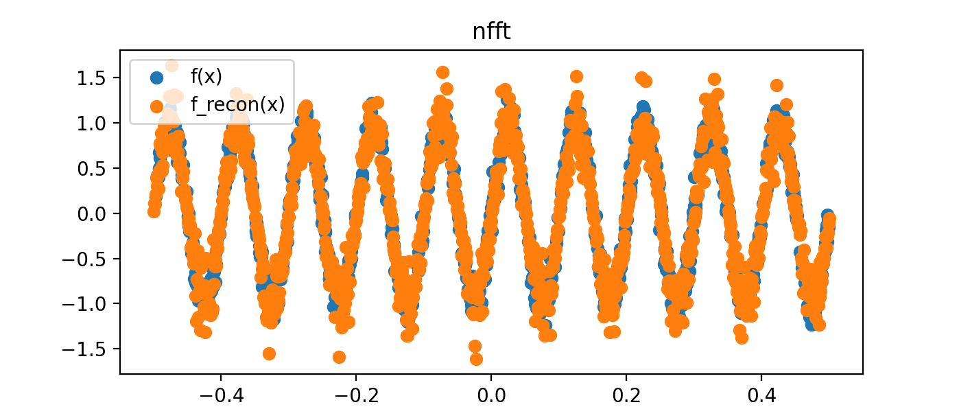
    plt.figure()
    plt.title('nfft')
    plt.scatter(x, f, label='f(x)')
    plt.scatter(x, f_recon, label='f_recon(x)', marker='+')
    plt.legend()

if True: #<--- Ensure non-global namespace
    #Define signal:
    x = numpy.linspace(-.5, .5, 1000)
    f = numpy.sin(10 * 2 * numpy.pi * x) + .1*numpy.random.randn( 1000 ) #Add some 'y' randomness to the sample

    #prepare wavenumbers for transform:
    N = len(x)
    TimeSpacing = x[1] - x[0]
    k = scipy.fft.fftfreq(N, TimeSpacing)
    #print ('k', k) #---> Confusing steps: [0,1,...500,-500,-499,...-1]
    
    f_k = scipy.fft.fft(f)

    #plot transform
    plt.figure()
    plt.plot(k, f_k.real, label='real')
    plt.plot(k, f_k.imag, label='imag')
    plt.legend()

    #Reconstruct the original signal with scipy.fft
    f_recon = scipy.fft.ifft(f_k)

    #Plot original vs reconstructed
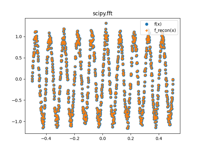
    plt.figure()
    plt.title('scipy.fft')
    plt.scatter(x, f, label='f(x)')
    plt.scatter(x, f_recon, label='f_recon(x)', marker='+')
    plt.legend()

plt.show()

以下是相关的生成地块：

​

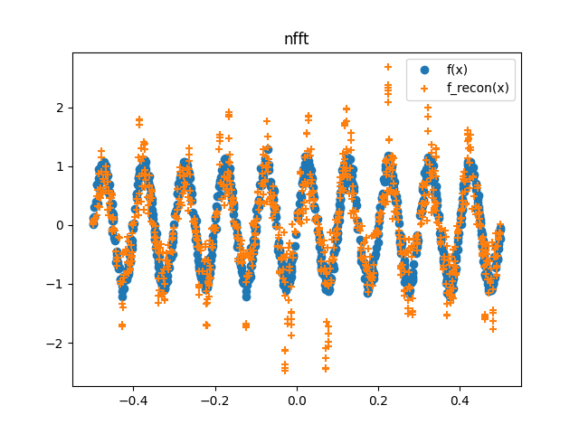
nfft的重建似乎在正常化方面失败了。我武断地把震级除以2000年，只是为了让它们更好地绘制出来。什么是正确的归一化常数？

nfft似乎也没有复制原来的观点。即使我的归一化常量是正确的，我也不可能得到原来的点。

我做错了什么，我该如何解决呢？

Answer 1

上面提到的包没有实现反向nfft。

ndft是f_hat @ np.exp(-2j * np.pi * x * k[:, None])，ndft_adjoint是f @ np.exp(2j * np.pi * k * x[:, None])

让k = -N//2 + np.arange(N)和A = np.exp(-2j * np.pi * k * k[:, None])

A @ np.conj(A) = N * np.eye(N) (数字检查)

因此，对于随机x，伴随变换等于逆变换。给出的参考文件提供了几个选项，我实现了算法1 CGNE，第9页

import numpy as np # I have the habit to use np
def nfft_inverse(x, y, N, w = 1, L=100):
    f = np.zeros(N, dtype=np.complex128);
    r = y - nfft.nfft(x, f);
    p = nfft.nfft_adjoint(x, r, N);
    r_norm = np.sum(abs(r)**2 * w)
    for l in range(L):
        p_norm = np.sum(abs(p)**2 * w);
        alpha = r_norm / p_norm
        f += alpha * w * p;
        r = y - nfft.nfft(x, f)
        r_norm_2 = np.sum(abs(r)**2 * w)
        beta = r_norm_2 / r_norm
        p = beta * p + nfft.nfft_adjoint(x, w * r, N)
        r_norm = r_norm_2;
        #print(l, r_norm)
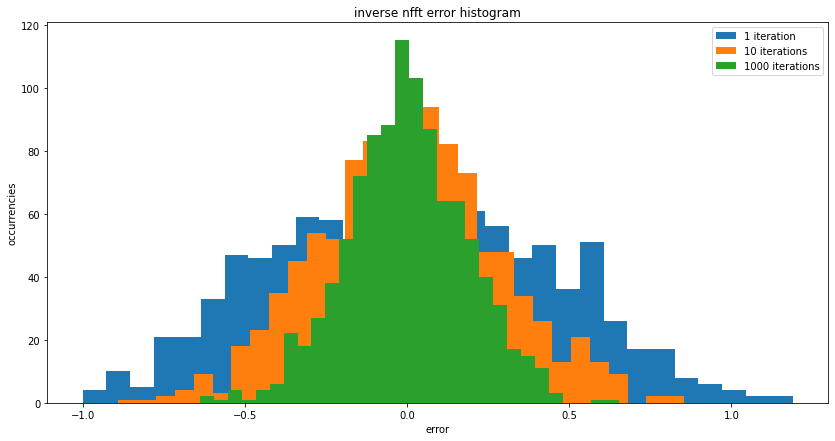
    return f;

该算法收敛速度慢，收敛速度差。

    plt.figure(figsize=(14, 7))
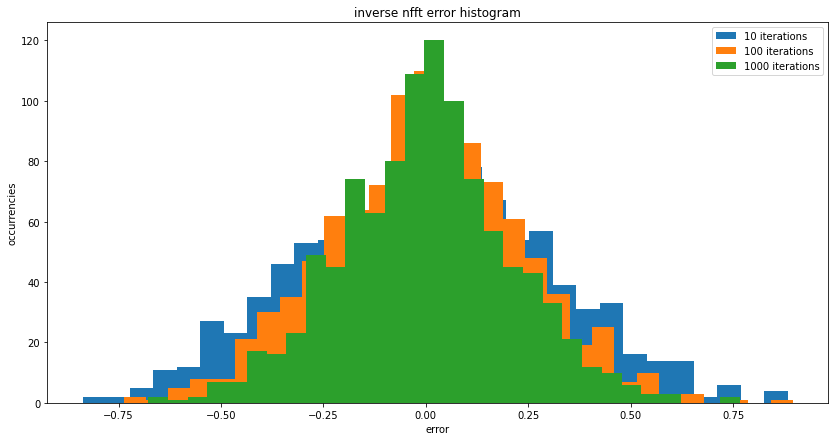
    plt.title('inverse nfft error histogram')
    #plt.scatter(x, f_hat, label='f(x)')
    h_hat = nfft_inverse(x, f, N, L = 1)
    plt.hist(f_hat - numpy.real(h_hat), bins=30, label='1 iteration')
    h_hat = nfft_inverse(x, f, N, L = 10)
    plt.hist(f_hat - numpy.real(h_hat), bins=30, label='10 iterations')
    h_hat = nfft_inverse(x, f, N, L = 1000)
    plt.hist(f_hat - numpy.real(h_hat), bins=30, label='1000 iterations')
    plt.xlabel('error')
    plt.ylabel('occurrencies')
    plt.legend()

​

​

我也尝试使用枕极小化，显式地最小化剩余的||nfft(x, f) - y||**2。

import numpy as np # the habit
import scipy.optimize
def nfft_gradient_descent(x, y, N, L=10, tol=1e-8, method='CG'):
    '''
    compute $min || A @ f - y ||**2 via gradient descent
    the gradient is
    
    `A^H @ (A @ f - y)`
    
    Multiply by A using nfft.nfft
    
    '''
    def cost(fpack):
        f = fpack[0::2] + 1j * fpack[1::2]
        u = np.sum(np.abs(nfft.nfft(x, f) - y)**2)
        return u
    def grad(fpack):
        f = fpack[0::2] + 1j * fpack[1::2]
        r = nfft.nfft(x, f) - y
        u = nfft.nfft_adjoint(x, r, N)
        return np.stack([np.real(u), np.imag(u)], axis=1).reshape(-1)
    
    x0 = np.zeros([N, 2])
    result = scipy.optimize.minimize(cost, x0=x0, jac=grad, tol=tol, method=method, options={'maxiter': L, 'disp': True})
    return result.x[0::2] + 1j * result.x[1::2];

结果看起来很相似，如果你愿意的话，你可以自己尝试不同的方法或参数。但我认为这种变换是病态的，因为变换后的残差大大减少了，但重构值上的残差却很大。

​

编辑1

从根本上说，你发现这个算法没有一个真正的反义词吗？我不能得到我的原点？X != nfft(nfft_adjoint(x))

请查看参考纸的2.3节

​

​

数值比较

Cris Luengo回答提供了另一种可能性，即，与其在x点重构f，不如使用ifft在等距点重构重放版本。所以你已经有三个选择了，我会做一个简单的比较。请记住，图中显示的是基于NFFT计算的16k样本，而这里我使用1k样本。

由于FFT方法使用不同的点，我们无法与原始信号进行比较，所以我要做的是在没有噪声的情况下与谐波函数进行比较。噪声的方差是0.01，所以精确的重构会导致这种均方误差。

N = 1024
x = -0.5 + numpy.random.rand(N)
f_hat = numpy.sin(10 * 2 * numpy.pi * x) + .1*numpy.random.randn( N ) #Add some  'y' randomness to the sample

k = - N // 2 + numpy.arange(N)
f = nfft.nfft(x, f_hat)

print('nfft_inverse')
h_hat = nfft_inverse(x, f, len(x), L = 10)
print('10 iterations: ', np.mean((numpy.sin(10 * 2 * numpy.pi * x) - numpy.real(h_hat))**2))
h_hat = nfft_inverse(x, f, len(x), L = 100)
print('100 iterations: ', np.mean((numpy.sin(10 * 2 * numpy.pi * x) - numpy.real(h_hat))**2))
h_hat = nfft_inverse(x, f, len(x), L = 1000)
print('1000 iterations: ', np.mean((numpy.sin(10 * 2 * numpy.pi * x) - numpy.real(h_hat))**2))
print('nfft_gradient_descent')
h_hat = nfft_gradient_descent(x, f, len(x), L = 10)
print('10 iterations: ', np.mean((numpy.sin(10 * 2 * numpy.pi * x) - numpy.real(h_hat))**2))
h_hat = nfft_gradient_descent(x, f, len(x), L = 100)
print('100 iterations: ', np.mean((numpy.sin(10 * 2 * numpy.pi * x) - numpy.real(h_hat))**2))
h_hat = nfft_gradient_descent(x, f, len(x), L = 1000)
print('1000 iterations: ', np.mean((numpy.sin(10 * 2 * numpy.pi * x) - numpy.real(h_hat))**2))


#Reconstruct the original at a spaced grid based on nfft result using ifft
f_recon = - numpy.fft.fftshift(numpy.fft.ifft(numpy.fft.ifftshift(f_k))) / (N / N2)
x_recon = k / N; 
print('using IFFT: ', np.mean((numpy.sin(10 * 2 * numpy.pi * x_recon) - numpy.real(f_recon))**2))

结果：

nfft_inverse
10 iterations:  0.0798988590351581
100 iterations:  0.05136853850272318
1000 iterations:  0.037316315280700896
nfft_gradient_descent
10 iterations:  0.08832834348902704
100 iterations:  0.05901599049633016
1000 iterations:  0.043921864589484
using IFFT:  0.49044932854606377

另一种看法是

plt.plot(numpy.sin(10 * 2 * numpy.pi * x_recon), numpy.real(f_recon), '.', label='ifft')
plt.plot(numpy.sin(10 * 2 * numpy.pi * x), numpy.real(nfft_gradient_descent(x, f, len(x), L = 5)), '.', label='gradient descent L=5')
plt.plot(numpy.sin(10 * 2 * numpy.pi * x), numpy.real(nfft_inverse(x, f, len(x), L = 5)), '.', label='nfft_inverse L=5')
plt.plot(numpy.sin(10 * 2 * numpy.pi * x), np.real(f_hat), '.', label='original')
plt.legend()

​

​

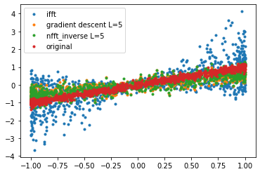
尽管IFFT矩阵具有更好的条件，但它给出的结果是信号的重建效果更差。此外，从最后的情节，它变得更加明显，有一个轻微的衰减。可能是由于系统的能量泄漏到假想部分(我的代码中有错误？？)。只是一个简单的测试，乘以1.3就可以得到更好的结果。

Answer 2

鲍勃已经发布了极好的回答，这只是为了补充一些细节，我希望是有益的。

首先，比较计算频率分量的两幅图。请注意，NFFT的噪声比常规FFT的噪声大得多。你估计这些频率分量的采样信号来自有噪声的样本，在一种情况下样本有规律的间隔，在另一种情况下它们是随机间隔的。这是一个众所周知的结果，常规抽样比随机抽样更有效(有效意味着你需要更少的样本来获取相同数量的信息)。因此，随机抽样会产生更多的噪声。

我们可以根据NFFT估计的频率分量计算“正常”逆FFT：

f_recon = numpy.fft.fftshift(numpy.fft.ifft(numpy.fft.ifftshift(f_k)))
x_recon = numpy.linspace(-.5, .5, N)

我使用ifftshift是因为NFFT定义了从-N/2到N/2-1的k，而FFT定义了从0到N-1。ifftshift交换信号的两部分，将第一部分转换为第二部分(从N/2到N-1的k等于-N/2到-1)。我还对IFFT的结果使用了fftshift，因为同样的东西适用于时间轴，它将原点从第一个样本移到序列的中间。

注意f_recon有多吵。我们可以用非均匀采样信号来解释f_k的差估计。还有一个符号错误，当我们比较f_k的两个估计值时，我们已经可以观察到这个错误。这来自于伴随的NFFT，指数中的符号与逆DFT相同，这实际上意味着f_recon是翻转的w.r.t。x。

如果我们增加随机样本的数量，我们可以得到一个更好的估计：

import numpy
import nfft
import matplotlib.pyplot as plt

#Define signal:
N = 1024 * 16  # power of two for speed
x = -0.5 + numpy.random.rand(N)
f = numpy.sin(10 * 2 * numpy.pi * x) + .1 * numpy.random.randn(N) # Add some  'y' randomness to the sample

#prepare wavenumbers for transform:
k = - N // 2 + numpy.arange(N) 

N2 = 1024
f_k = nfft.nfft_adjoint(x, f, N2, truncated=False)

#Reconstruct the original signal with nfft
#   (note the minus sign to flip the signal, in reality we should flip x)
f_recon = - numpy.fft.fftshift(numpy.fft.ifft(numpy.fft.ifftshift(f_k))) / (N / N2)
x_recon = numpy.linspace(-.5, .5, N2, endpoint=False)

#Plot original vs reconstructed
plt.figure()
plt.title('nfft')
plt.scatter(x[:N2], f[:N2], label='f(x)') # don't plot all samples, there's too many
plt.scatter(x_recon, f_recon, label='f_recon(x)')
plt.legend()
plt.show()

​

​