tf.keras中线性回归模型调优的几个问题

Question

我正在开发用综合数据Colab练习进行线性回归，它使用一个玩具数据集探索线性回归。建立并训练了一个线性回归模型，它与学习速度、时间和批次大小有关。我很难理解迭代是如何完成的，它是如何连接到“时代”和“批处理大小”的。我基本上不知道实际的模型是如何训练的，数据是如何处理的，迭代是如何完成的。为了理解这一点，我想通过手工计算每一步来遵循这一点。因此，我希望每一步都有斜率和截距系数。这样我就可以看到“计算机”使用什么样的数据，把什么样的数据放入模型中，在每一次特定的迭代中得到什么样的模型结果，以及迭代是如何完成的。我首先尝试获取每个步骤的斜率和拦截，但是失败了，因为只有在最后才输出斜率和截距。我修改的代码(原件，刚刚添加：)

  print("Slope")
  print(trained_weight)
  print("Intercept")
  print(trained_bias)

代码：

import pandas as pd
import tensorflow as tf
from matplotlib import pyplot as plt

#@title Define the functions that build and train a model
def build_model(my_learning_rate):
  """Create and compile a simple linear regression model."""
  # Most simple tf.keras models are sequential. 
  # A sequential model contains one or more layers.
  model = tf.keras.models.Sequential()

  # Describe the topography of the model.
  # The topography of a simple linear regression model
  # is a single node in a single layer. 
  model.add(tf.keras.layers.Dense(units=1, 
                                  input_shape=(1,)))

  # Compile the model topography into code that 
  # TensorFlow can efficiently execute. Configure 
  # training to minimize the model's mean squared error. 
  model.compile(optimizer=tf.keras.optimizers.RMSprop(lr=my_learning_rate),
                loss="mean_squared_error",
                metrics=[tf.keras.metrics.RootMeanSquaredError()])
 
  return model           


def train_model(model, feature, label, epochs, batch_size):
  """Train the model by feeding it data."""

  # Feed the feature values and the label values to the 
  # model. The model will train for the specified number 
  # of epochs, gradually learning how the feature values
  # relate to the label values. 
  history = model.fit(x=feature,
                      y=label,
                      batch_size=batch_size,
                      epochs=epochs)

  # Gather the trained model's weight and bias.
  trained_weight = model.get_weights()[0]
  trained_bias = model.get_weights()[1]
  print("Slope")
  print(trained_weight)
  print("Intercept")
  print(trained_bias)
  # The list of epochs is stored separately from the 
  # rest of history.
  epochs = history.epoch

  # Gather the history (a snapshot) of each epoch.
  hist = pd.DataFrame(history.history)

 # print(hist)
  # Specifically gather the model's root mean 
  #squared error at each epoch. 
  rmse = hist["root_mean_squared_error"]

  return trained_weight, trained_bias, epochs, rmse

print("Defined create_model and train_model")

#@title Define the plotting functions
def plot_the_model(trained_weight, trained_bias, feature, label):
  """Plot the trained model against the training feature and label."""

  # Label the axes.
  plt.xlabel("feature")
  plt.ylabel("label")

  # Plot the feature values vs. label values.
  plt.scatter(feature, label)

  # Create a red line representing the model. The red line starts
  # at coordinates (x0, y0) and ends at coordinates (x1, y1).
  x0 = 0
  y0 = trained_bias
  x1 = my_feature[-1]
  y1 = trained_bias + (trained_weight * x1)
  plt.plot([x0, x1], [y0, y1], c='r')

  # Render the scatter plot and the red line.
  plt.show()

def plot_the_loss_curve(epochs, rmse):
  """Plot the loss curve, which shows loss vs. epoch."""

  plt.figure()
  plt.xlabel("Epoch")
  plt.ylabel("Root Mean Squared Error")

  plt.plot(epochs, rmse, label="Loss")
  plt.legend()
  plt.ylim([rmse.min()*0.97, rmse.max()])
  plt.show()

print("Defined the plot_the_model and plot_the_loss_curve functions.")

my_feature = ([1.0, 2.0,  3.0,  4.0,  5.0,  6.0,  7.0,  8.0,  9.0, 10.0, 11.0, 12.0])
my_label   = ([5.0, 8.8,  9.6, 14.2, 18.8, 19.5, 21.4, 26.8, 28.9, 32.0, 33.8, 38.2])

learning_rate=0.05
epochs=1
my_batch_size=12

my_model = build_model(learning_rate)
trained_weight, trained_bias, epochs, rmse = train_model(my_model, my_feature, 
                                                         my_label, epochs,
                                                         my_batch_size)
plot_the_model(trained_weight, trained_bias, my_feature, my_label)
plot_the_loss_curve(epochs, rmse)

在我的具体情况下，我的输出是：

​

​

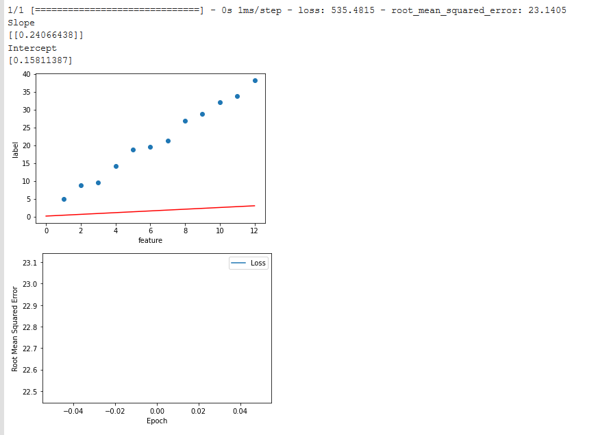
现在，我尝试在一个简单的excel表中复制这一点，并手动计算rmse：

​

​

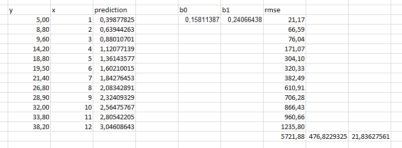
然而，我得到了21.8而不是23.1？而且我的损失不是535.48，而是476.82

因此，我的第一个问题是:我的错误在哪里，如何计算rmse？

第二个问题:如何获得每个特定迭代的rmse？让我们考虑时代是4，批大小是4。

​

​

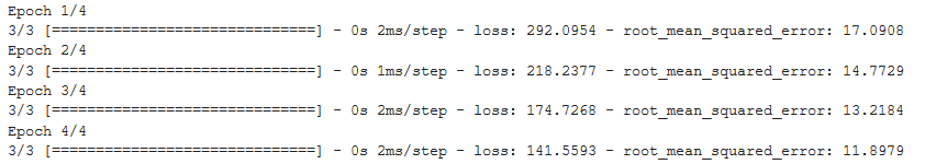
这给出了4个年代和3个批次，每4个例子(观察)。我不明白这些迭代是如何训练模型的。那么，如何才能得到每个回归模型和rmse的系数？不只是每个时代(so 4)，而是每一次迭代。我认为每个时代都有3次迭代。那么，我认为总共有12个线性回归模型的结果？我想看看这12位模特。在没有提供信息的情况下，起始点的初始值是多少，使用了什么样的斜率和截距？从真正的第一点开始。我没有具体说明这一点。然后，我想能够跟踪斜率和拦截是如何适应每一步。这将是从梯度下降算法，我认为。但那将是超级加号。对我来说，更重要的是首先了解这些迭代是如何完成的，以及它们是如何连接到时代和批处理的。

更新:我知道初始值(对于斜率和截距)是随机选择的。

Answer 1

基础

问题陈述

让我们考虑一组样本X的线性回归模型，其中每个样本都由一个特征x表示。作为模型训练的一部分，我们正在搜索线w.x + b，使((w.x+b) -y )^2 (平方损失)最小。对于一组数据点，我们取每个样本的平方损失的平均值，也就是所谓的均方误差(MSE)。表示重量和偏倚的w和b统称为权重。

拟合线/训练模型

1. 我们有一个解线性回归问题的封闭形式的解，它是(X^T.X)^-1.X^T.y。
2. 我们也可以使用梯度体面的方法来寻找权重，以最小化平方损失。像tensorflow这样的框架使用梯度体面来搜索权重(称为训练)。

梯度体面

一种学习回归的梯度体面算法看起来像是打击。

w, b = some initial value
While model has not converged:
    y_hat = w.X + b
    error = MSE(y, y_hat) 
    back propagate (BPP) error and adjust weights

上述循环的每一次运行都被称为一个时代。然而，由于资源的限制，y_hat、error和BPP的计算并不是在完整的数据集上预先准备好的，而是将数据划分成较小的批，并且每次只对一批进行上述操作。此外，我们通常确定时间的数目，并监测模型是否已经收敛。

w, b = some initial value
for i in range(number_of_epochs)
    for X_batch,y_batch in get_next_batch(X, y)
        y_hat = w.X_batch + b
        error = MSE(y_batch, y_hat) 
    back propagate (BPP) error and adjust weights

批处理的Keras实现

让我们说，我们想要添加根均方误差，以跟踪模型的性能，而它是培训。Keras实现的方式如下

w, b = some initial value
for i in range(number_of_epochs)
    all_y_hats = []
    all_ys = []
    for X_batch,y_batch in get_next_batch(X, y)
        y_hat = w.X_batch + b
        error = MSE(y_batch, y_hat)

        all_y_hats.extend(y_hat) 
        all_ys.extend(y_batch)

        batch_rms_error = RMSE(all_ys, all_y_hats)

    back propagate (BPP) error and adjust weights

正如您在上面看到的，预测是累积的，RMSE是根据累积的预测来计算的，而不是所有以前的批RMSE的平均值。

在keras中的实现

现在我们的基础已经清楚了，让我们看看如何在keras中实现同样的跟踪。keras有回调，因此我们可以连接到on_batch_begin回调并积累all_y_hats和all_ys。在on_batch_end上，回调角给出了计算出的RMSE。我们将使用累积的RMSE和all_ys手动计算all_y_hats，并验证它是否与keras计算的内容相同。我们还将节省重量，以便以后可以画出正在学习的线。

import numpy as np
from sklearn.metrics import mean_squared_error
import keras
import matplotlib.pyplot as plt

# Some training data
X = np.arange(16)
y = 0.5*X +0.2

batch_size = 8
all_y_hats = []
learned_weights = [] 

class CustomCallback(keras.callbacks.Callback):
  def on_batch_begin(self, batch, logs={}):    
    w = self.model.layers[0].weights[0].numpy()[0][0]
    b = self.model.layers[0].weights[1].numpy()[0]    
    s = batch*batch_size
    all_y_hats.extend(b + w*X[s:s+batch_size])    
    learned_weights.append([w,b])

  def on_batch_end(self, batch, logs={}):    
    calculated_error = np.sqrt(mean_squared_error(all_y_hats, y[:len(all_y_hats)]))
    print (f"\n Calculated: {calculated_error},  Actual: {logs['root_mean_squared_error']}")
    assert np.isclose(calculated_error, logs['root_mean_squared_error'])

  def on_epoch_end(self, batch, logs={}):
    del all_y_hats[:]    


model = keras.models.Sequential()
model.add(keras.layers.Dense(1, input_shape=(1,)))
model.compile(optimizer=keras.optimizers.RMSprop(lr=0.01), loss="mean_squared_error",  metrics=[keras.metrics.RootMeanSquaredError()])
# We should set shuffle=False so that we know how baches are divided
history = model.fit(X,y, epochs=100, callbacks=[CustomCallback()], batch_size=batch_size, shuffle=False) 

输出：

Epoch 1/100
 8/16 [==============>...............] - ETA: 0s - loss: 16.5132 - root_mean_squared_error: 4.0636
 Calculated: 4.063645694548688,  Actual: 4.063645839691162

 Calculated: 8.10112834945773,  Actual: 8.101128578186035
16/16 [==============================] - 0s 3ms/step - loss: 65.6283 - root_mean_squared_error: 8.1011
Epoch 2/100
 8/16 [==============>...............] - ETA: 0s - loss: 14.0454 - root_mean_squared_error: 3.7477
 Calculated: 3.7477213352845675,  Actual: 3.7477214336395264
-------------- truncated -----------------------

塔-达！断言assert np.isclose(calculated_error, logs['root_mean_squared_error'])从未失败，因此我们的计算/理解是正确的。

线

最后，以均方误差损失为基础，绘制BPP算法调整的直线。我们可以使用下面的代码创建一个png图像，每批正在学习的线路连同列车数据。

for i, (w,b) in enumerate(learned_weights):
  plt.close()
  plt.axis([-1, 18, -1, 10])
  plt.scatter(X, y)
  plt.plot([-1,17], [-1*w+b, 17*w+b], color='green')
  plt.savefig(f'img{i+1}.png')

下面是按学习顺序排列的上述图像的gif动画。

​

​

当y = 0.5*X +5.2时正在学习的超平面(在本例中为行)

​

​

Answer 2

我试着玩它，我认为它是这样的：

1. 初始化每个功能的权重(通常是随机的，取决于设置)。另外，初始为0.0的偏差也被启动。
2. 第一批的损失和度量是计算和打印的，权重和偏差被更新。
3. 步骤2在所有批中重复，然而，在上次批处理丢失后的和度量没有被打印，所以您在屏幕上看到的是在时代中上次更新之前所看到的丢失和度量。
4. 新的时代已经开始，你看到的第一次度量和损失，实际上是根据上一次更新的权数计算的。

所以基本上，我认为直觉地说，首先计算损失，然后更新权重，这意味着权值更新是时代的最后一次运算。

如果您的模型使用一个时代和一个批训练，那么您在屏幕上看到的是根据初始权重和偏差计算的损失。如果您希望看到每个时代结束后的损失和度量(具有大多数“实际”权重)，则可以将参数validation_data=(X,y)传递给fit方法。这将告诉算法在完成once时，再一次计算这个给定验证数据的损失和度量。

关于模型的初始权重，当您手动为层设置一些初始权重时(使用kernel_initializer参数)，您可以尝试它：

  model.add(tf.keras.layers.Dense(units=1,
                                  input_shape=(1,),
                                  kernel_initializer=tf.constant_initializer(.5)))

下面是train_model函数的更新部分，它显示了我的意思：

  def train_model(model, feature, label, epochs, batch_size):
        """Train the model by feeding it data."""

        # Feed the feature values and the label values to the
        # model. The model will train for the specified number
        # of epochs, gradually learning how the feature values
        # relate to the label values.
        init_slope = model.get_weights()[0][0][0]
        init_bias = model.get_weights()[1][0]
        print('init slope is {}'.format(init_slope))
        print('init bias is {}'.format(init_bias))

        history = model.fit(x=feature,
                          y=label,
                          batch_size=batch_size,
                          epochs=epochs,
                          validation_data=(feature,label))

        # Gather the trained model's weight and bias.
        #print(model.get_weights())
        trained_weight = model.get_weights()[0]
        trained_bias = model.get_weights()[1]
        print("Slope")
        print(trained_weight)
        print("Intercept")
        print(trained_bias)
        # The list of epochs is stored separately from the
        # rest of history.
        prediction_manual = [trained_weight[0][0]*i + trained_bias[0] for i in feature]

        manual_loss = np.mean(((np.array(label)-np.array(prediction_manual))**2))
        print('manually computed loss after slope and bias update is {}'.format(manual_loss))
        print('manually computed rmse after slope and bias update is {}'.format(manual_loss**(1/2)))

        prediction_manual_init = [init_slope*i + init_bias for i in feature]
        manual_loss_init = np.mean(((np.array(label)-np.array(prediction_manual_init))**2))
        print('manually computed loss with init slope and bias is {}'.format(manual_loss_init))
        print('manually copmuted loss with init slope and bias is {}'.format(manual_loss_init**(1/2)))

产出：

"""
init slope is 0.5
init bias is 0.0
1/1 [==============================] - 0s 117ms/step - loss: 402.9850 - root_mean_squared_error: 20.0745 - val_loss: 352.3351 - val_root_mean_squared_error: 18.7706
Slope
[[0.65811384]]
Intercept
[0.15811387]
manually computed loss after slope and bias update is 352.3350379264957
manually computed rmse after slope and bias update is 18.77058970641295
manually computed loss with init slope and bias is 402.98499999999996
manually copmuted loss with init slope and bias is 20.074486294797182
"""

注意，在斜率和偏差更新后手工计算的损失和度量与验证损失和度量匹配，更新前手工计算的损失和度量匹配初始斜率和偏差的损失和度量。

关于第二个问题，我认为您可以手动将数据分成几个批次，然后对每一批进行迭代并放入其中。然后，在每次迭代中，模型输出验证数据的损失和度量。就像这样：

  init_slope = model.get_weights()[0][0][0]
  init_bias = model.get_weights()[1][0]
  print('init slope is {}'.format(init_slope))
  print('init bias is {}'.format(init_bias))
  batch_size = 3

  for idx in range(0,len(feature),batch_size):
      model.fit(x=feature[idx:idx+batch_size],
                y=label[idx:idx+batch_size],
                batch_size=1000,
                epochs=epochs,
                validation_data=(feature,label))
      print('slope: {}'.format(model.get_weights()[0][0][0]))
      print('intercept: {}'.format(model.get_weights()[1][0]))
      print('x data used: {}'.format(feature[idx:idx+batch_size]))
      print('y data used: {}'.format(label[idx:idx+batch_size]))

产出：

init slope is 0.5
init bias is 0.0
1/1 [==============================] - 0s 117ms/step - loss: 48.9000 - root_mean_squared_error: 6.9929 - val_loss: 352.3351 - val_root_mean_squared_error: 18.7706
slope: 0.6581138372421265
intercept: 0.15811386704444885
x data used: [1.0, 2.0, 3.0]
y data used: [5.0, 8.8, 9.6]
1/1 [==============================] - 0s 21ms/step - loss: 200.9296 - root_mean_squared_error: 14.1750 - val_loss: 306.3082 - val_root_mean_squared_error: 17.5017
slope: 0.8132714033126831
intercept: 0.3018075227737427
x data used: [4.0, 5.0, 6.0]
y data used: [14.2, 18.8, 19.5]
1/1 [==============================] - 0s 22ms/step - loss: 363.2630 - root_mean_squared_error: 19.0595 - val_loss: 266.7119 - val_root_mean_squared_error: 16.3313
slope: 0.9573485255241394
intercept: 0.42669767141342163
x data used: [7.0, 8.0, 9.0]
y data used: [21.4, 26.8, 28.9]
1/1 [==============================] - 0s 22ms/step - loss: 565.5593 - root_mean_squared_error: 23.7815 - val_loss: 232.1553 - val_root_mean_squared_error: 15.2366
slope: 1.0924618244171143
intercept: 0.5409283638000488
x data used: [10.0, 11.0, 12.0]
y data used: [32.0, 33.8, 38.2]

Answer 3

线性回归模型

线性回归模型只有一个具有线性激活函数的神经元。关于培训的基础模型是我们使用梯度下降。每次整个数据通过模型并更新权重时，就称为1纪元。然而，迭代和时代的概念在这里并没有什么不同。

基本培训步骤

Prepare data
Initialize the model and its parameters (weights and biases)
for each epoch:  #(both iteration and epoch same here)
    Forward Propagation
    Compute Cost
    Back Propagation
    Update Parameters

梯度下降有三个变体

• 分批梯度下降(BDG)
• 随机梯度下降(SDG)
• 小批量梯度下降(千年发展目标)

批处理梯度下降是我们前面讨论过的(传递整个数据)。通常也称为梯度下降。

在随机梯度下降中，我们一次传递一个随机例子，并根据传递的每一个例子更新权重。现在，迭代开始发挥作用。在训练完成后，以1例为例，完成了1迭代。然而，在数据集中有更多的模型尚未看到的例子。完全训练所有这些例子称为1纪元。由于一次传递一个示例，SDG对于较大的数据集非常慢，因为它失去了向量化的效果。

因此，我们通常使用最小批处理梯度下降.在这里，数据集被划分为一些固定大小的块。每个数据块的大小称为批处理大小，它可以介于1和数据大小之间。在每个时代，这些批次的数据被用来训练模型。

1迭代处理1批数据。一个时代处理整批数据。一个纪元包含一个或多个迭代。

因此，如果数据的大小为m，则在每次迭代期间输入的数据如下：

• BDG =m
• SDG =1
• 千年发展目标=1

MGD的基本培训步骤

Prepare data
Initialize the model and its parameters (weights and biases)
for each epoch:  #(epoch)
    for each mini_batch: #(iteration)
        Forward Propagation
        Compute Cost
        Back Propagation
        Update Parameters

这是梯度下降、批量、时代和迭代背后的理论概念。

现在转到Keras和您的代码：

我给你查了柯拉码，它运行得很好。在您已经发布的代码中，纪元的数量是1，这对于模型来说是非常小的，因为数据非常少，而且模型本身非常简单。因此，您需要增加、增加数据量、或，创建更复杂的模型、或列车，以便为更多的纪元提供更多的数据，从我从笔记本中找到的400-500个。只要适当调整学习速度，就可以减少学习次数。

learning_rate=0.14
epochs=70
my_batch_size= 32 

my_model = build_model(learning_rate)
trained_weight, trained_bias, epochs, rmse = train_model(my_model, my_feature, 
                                                        my_label, epochs,
                                                        my_batch_size)
plot_the_model(trained_weight, trained_bias, my_feature, my_label)
plot_the_loss_curve(epochs, rmse)

当学习率很小时，模型学习速度较慢，因此需要较大的训练周期(Epoch)来进行更准确的预测。随着学习速度的提高，学习过程加快，从而缩短了学习周期。请比较colab中代码的不同部分，以获得适当的示例。

关于每次迭代的度量：

Keras是TensorFlow的高级API .到目前为止，我知道(不考虑API的定制)，在Keras的培训期间，它在每次迭代结束时计算训练集的损失、错误和准确性，并在每个时代结束时返回它们各自的平均值。因此，如果存在n历元，那么无论其间有多少次迭代，这些度量中的每一个都会有n数。

关于坡度和截距：

线性回归模型在输出层采用线性激活函数，即y = mx + c。我们所拥有的价值

• Y-指输出
• X-指输入
• M-指必须调整的坡度。
• C-指拦截(也可以调整)

在我们的模型中，这些m和c是我们调整的。它们是我们模型的重量和偏见。因此，我们的函数类似于y = Wx + b，其中b给出了截距，w给出了斜率。在开始时随机初始化权重和偏差。

从零开始线性回归模型的Colab链接

请根据需要调整值。由于模型是从零开始实现的，所以收集或打印在培训期间要跟踪的任何值。您也可以使用您自己的数据集，但是要确保它是有效的，或者是由某个库生成的，以便进行模型验证(Sklearn)。

0xBHq?usp=sharing

如果你觉得有什么让人费解的地方，请评论。我很乐意回答。