基于xarray-regrid对ERA5数据进行多种插值方法绘图对比

!pip install xarray_regrid

import xarray as xr
import xarray_regrid
from xarray_regrid import Grid
import matplotlib.pyplot as plt
import cartopy.crs as ccrs
import cartopy.feature as cfeature
from time import time
import numpy as np

new_grid = Grid(
    north=54,       # 北边界
    south=18,       # 南边界
    west=73,        # 西边界
    east=135,       # 东边界
    resolution_lat=0.05,  # 纬度分辨率
    resolution_lon=0.05   # 经度分辨率
)
target_ds = new_grid.create_regridding_dataset()

# 加载ERA5数据
ds = xr.open_dataset("/home/mw/input/era5sample8008/era5.nc")
# 选择一个时间点进行测试
ds = ds.isel(time=0)
lon_min, lon_max = 73, 135
lat_min, lat_max = 18, 54

ds = ds.sel(
    longitude=slice(lon_min, lon_max),
    latitude=slice(lat_max, lat_min)  
# 定义所有插值方法
methods = [
    ('linear', '线性插值'),
    ('nearest', '最近邻插值'),
    ('conservative', '保守插值'),
    ('cubic', '三次插值')

]

# 创建绘图
fig = plt.figure(figsize=(12, 20),dpi=200)
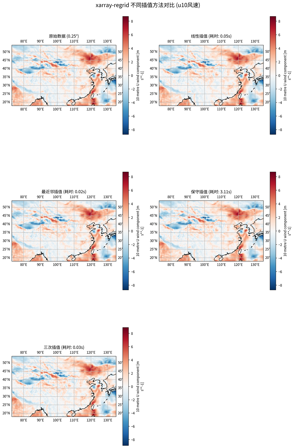
fig.suptitle('xarray-regrid 不同插值方法对比 (u10风速)', fontsize=16, y=0.95)

# 原始数据绘图
ax = fig.add_subplot(3, 2, 1, projection=ccrs.PlateCarree())
ds['u10'].plot(ax=ax, transform=ccrs.PlateCarree(), 
              cbar_kwargs={'shrink': 0.7})
ax.set_title('原始数据 (0.25°)')
ax.coastlines()
ax.gridlines(draw_labels=True)

# 执行所有插值方法并绘图
results = {}
for i, (method, title) in enumerate(methods, start=2):
    t_start = time()
    


    regridded_ds = getattr(ds.regrid, method)(target_ds)
    
    regridded_ds = regridded_ds.compute()
    elapsed = time() - t_start
    
    # 存储结果
    results[method] = {
        'data': regridded_ds,
        'time': elapsed
    }
    
    # 绘图
    ax = fig.add_subplot(3, 2, i, projection=ccrs.PlateCarree())
    regridded_ds['u10'].plot(ax=ax, transform=ccrs.PlateCarree(),
                           cbar_kwargs={'shrink': 0.7})
    ax.set_title(f'{title} (耗时: {elapsed:.2f}s)')
    ax.coastlines()
    ax.gridlines(draw_labels=True)

plt.tight_layout()
plt.show()

# 输出统计信息
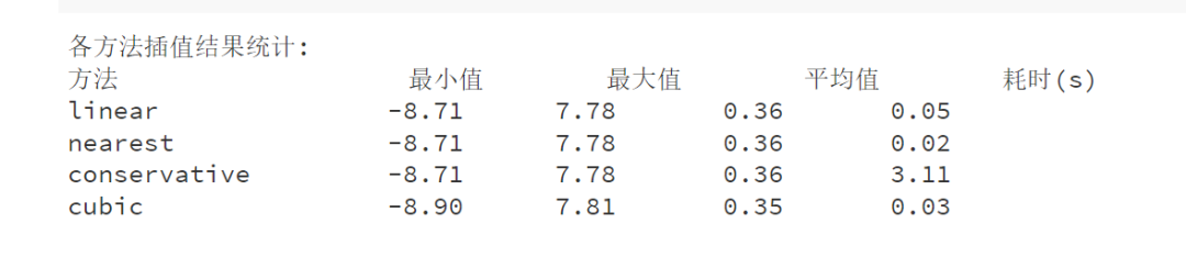
print("\n各方法插值结果统计:")
print("{:<20} {:<10} {:<10} {:<10} {:<10}".format(
    "方法", "最小值", "最大值", "平均值", "耗时(s)"))
for method, result in results.items():
    data = result['data']['u10']
    print("{:<20} {:<10.2f} {:<10.2f} {:<10.2f} {:<10.2f}".format(
        method, float(data.min()), float(data.max()), 
        float(data.mean()), result['time']))