你们用算法算遍了一切,就是没算到我不要命


这飞驰人生都三部了,但是我就记得俩部。。。没事,昨晚补上了。
这部片子除了热血以外也是告诉普罗大众一些道理,为什么张弛不走更好走的南线,是因为南线车>人,在柏油路上车好就是跑的快,而在北线就有了非常多的不确定性,入弯可能快 2 秒,一次失误就翻车,更多考验的是真真正正的车技;这是普通的无奈之举。(但是现在顶级拉力赛也不让混动车和油车一起跑)
在电影的最开始其实闪过几行诗,依稀记得小时候还背过,当年还真的以为是作者在走路,20 多年后再看,这路居然在每个人的脚下。
黄色的树林里分出两条路, 可惜我不能同时去涉足, 我在那路口久久伫立, 我向着一条路极目望去, 直到它消失在丛林深处。 但我选择了另一条路, 它荒草萋萋,十分幽寂, 显得更诱人,更美丽; 虽然在这两条道路上, 都留下了过往的足迹。 那天清晨落叶满地, 两条路都未经脚印污染。 啊,我把第一条路留待他日! 但我知道路径延绵无尽头, 恐怕我再也不会回返。 也许多少年后在某个地方, 我将轻声叹息将往事回顾: 一片树林里分出两条路, 而我选择了人迹更少的那条, 从此决定了我一生的道路。
没钱没资源,就是要走不确定性大的路。
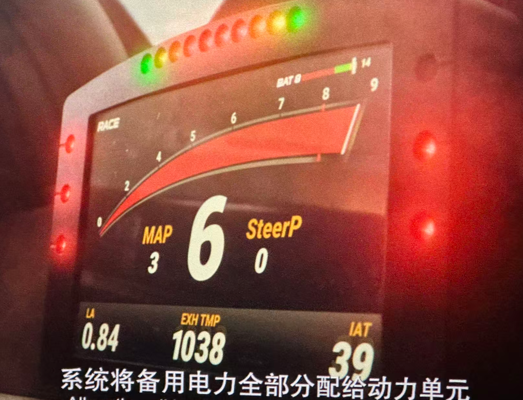
说起来这个不确定性,就引入这个 AI 的话题吧;里面这个编号也是耐人寻味,SS1 直接到 SS8,在什么路面都能判断,大雾天还出现了高斯什么?(但是一看就是高斯泼溅这种东西)好像是在屏幕上面模拟了一条赛道出来,属于 AR(增强现实的一种)。然后后面张弛入弯的时候有个最佳的入弯点,张弛凭经验是更晚入弯,也成功了,AI 直接说比不了,还得学习。。。在人类长期主导的专业领域如赛车运动中,AI究竟能否突破人类经验积累的“极限”?还是说,它更像一种保守的“安全选项”—能确保不错,却难以成就卓越?(甚至在最后都让对手把转速拉满,AI 觉得不行,张弛觉得可以),在人类文明的发展,往往依赖于敢于冒险、打破常规、超越自我设限的精神。AI是否可能具备这种“主动寻求突破”的意志?还是说,它的“突破”永远只能建立在人类预设的算法与数据框架之内?更进一步说,如果未来某天AI真的获得了某种“突破极限”的意愿与能力,那么人类在其中将扮演怎样的角色?是引导者、竞争者,还是逐渐被超越的“旧范式”?当AI开始追求自我超越时,人类存在的意义又该如何锚定?
人类的不确定性永远就是最大的惊喜,这种突如其来的热血,就是最大的翻盘机会,
最让我记住的是一个转场,谁说中国没有好转场的!
太帅了~
太帅了~
另外,夜晚,赛车,烟火,也是顶级的浪漫:

像是半路的赞歌
像是半路的赞歌
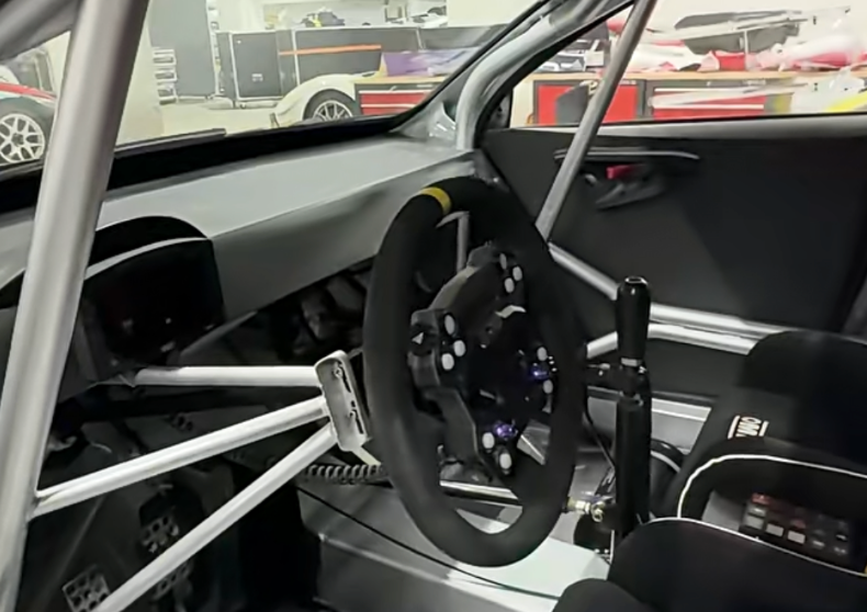
聊聊车
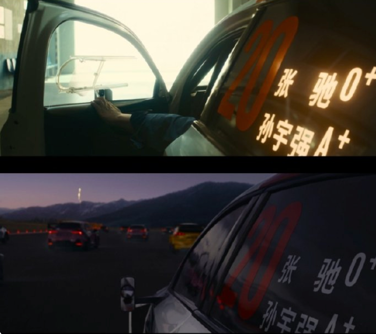
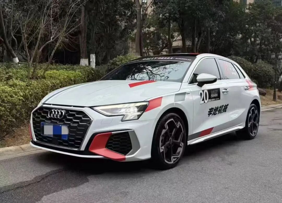
虽然我今年才拿到驾驶证,才开了几百公里,但是面对引擎的轰鸣,我也仍然兴奋。hhhh;其中主角奥迪A3这一台车,成本就超过了 550万人民币;除了外观,更多改造是在操控性能上的升级。(A3 就是一个壳子)
2 厢车
2 厢车
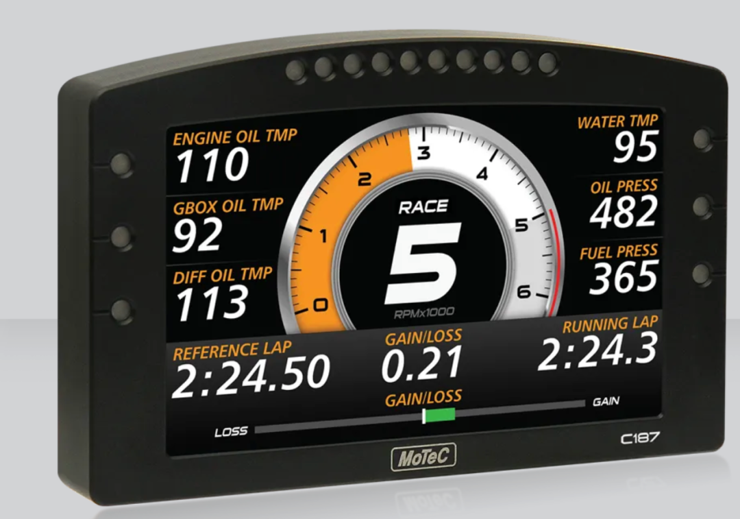
比如:对2.0T发动机进行深度强化,使马力超过300匹,扭矩超500牛·米,并匹配了换挡速度极快的序列式变速箱。这台车还装载了可调式绞牙避震、OMP赛车方向盘和桶形座椅、五点式安全带,以及能显示上百项数据的MoTeC专业仪表盘。
就是这个了
就是这个了
然后这个应该是混动的车
然后这个应该是混动的车
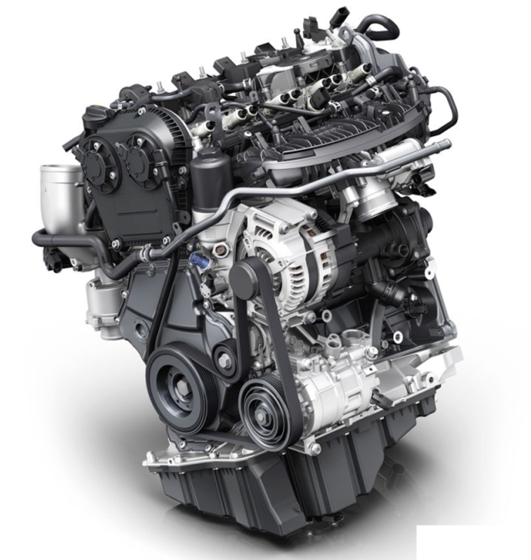
EA888 发动机!!!而且安装位置全部调整,估计是重量的问题;EA888 被誉为“改装神机”。仅通过 ECU 软件优化(一阶)即可提升 30-70 匹马力;三阶改装可轻松突破 450-500 匹;另外也可以通过改变进气门关闭时机实现高压缩比膨胀,在保证扭矩的同时显著降低油耗,其中三代机型通过减薄缸体厚度 0.5mm、减少曲轴配重块(8 变 4)等手段,大幅降低了整机重量。
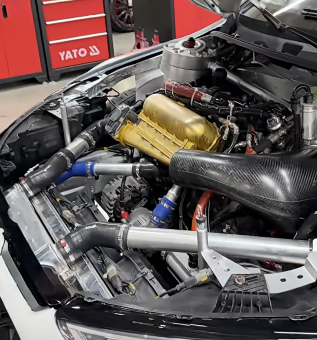
image-20260226153541373
大众 EA888 发动机是大众汽车集团(VAG)旗下的核心动力单元,自 2004 年诞生以来已历经五代进化。它广泛应用于大众、奥迪、保时捷、斯柯达等品牌的 1.8T 和 2.0T 车型中。
第一代 (Gen 1, 2006-2009):引入了缸内直喷、涡轮增压、双平衡轴及水冷技术。
第二代 (Gen 2, 2009-2012):加入了 AVS(奥迪气门升程系统),提升了扭矩表现。但此代因活塞环设计缺陷和油气分离器效率低,导致严重的烧机油和积碳问题。
第三代 (Gen 3, 2011 亮相):目前市场主流。采用了 FSI+MPI 双喷射系统(部分型号)和缸盖集成排气歧管,有效解决了烧机油通病,且热车速度更快。
第四代 (Gen 4 / EVO4):进一步优化排放与动力。更换了涡轮供应商(由 IHI 变为 Garrett/Continental),配备了更精确的电子泄压阀,最大功率可达 333 匹马力。
第五代 (Gen 5):于 2025 年正式亮相,由上汽大众途昂 Pro 首发搭载,重点针对混动系统进行适配。
哒哒哒
哒哒哒
当然了,奥迪已经赢到 WRC 不让上了,hhhh
有了心脏,当然要有一套强大的动力传输系统!所以要配个变速箱,这里也是奥迪旗下自己的系统:
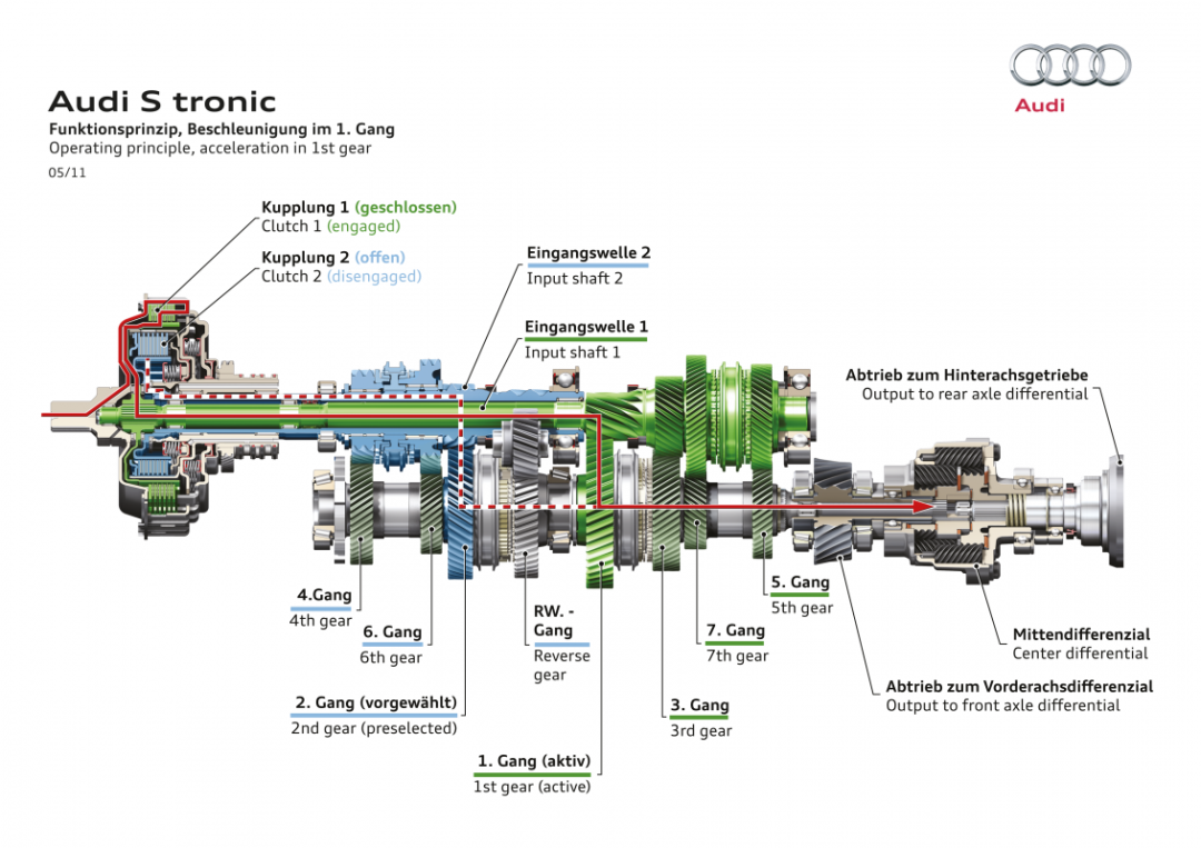
S-Tronic:双离合变速箱
S-Tronic 是奥迪(Audi)对其双离合变速箱(Dual-Clutch Transmission, DCT)技术的商业称呼;它本质上与大众的 DSG 变速箱技术相同,但针对奥迪的纵置或横置发动机布局进行了专门优化。
S-Tronic 拥有两组独立工作的离合器:一组离合器控制奇数挡(1、3、5、7),另一组控制偶数挡(2、4、6)和倒挡;当驾驶员在当前挡位行驶时,另一组离合器已经预先挂好了下一个逻辑挡位;换挡时,一组离合器瞬间分离,另一组同时接合,过程仅需约 0.2 秒,几乎感觉不到动力中断。
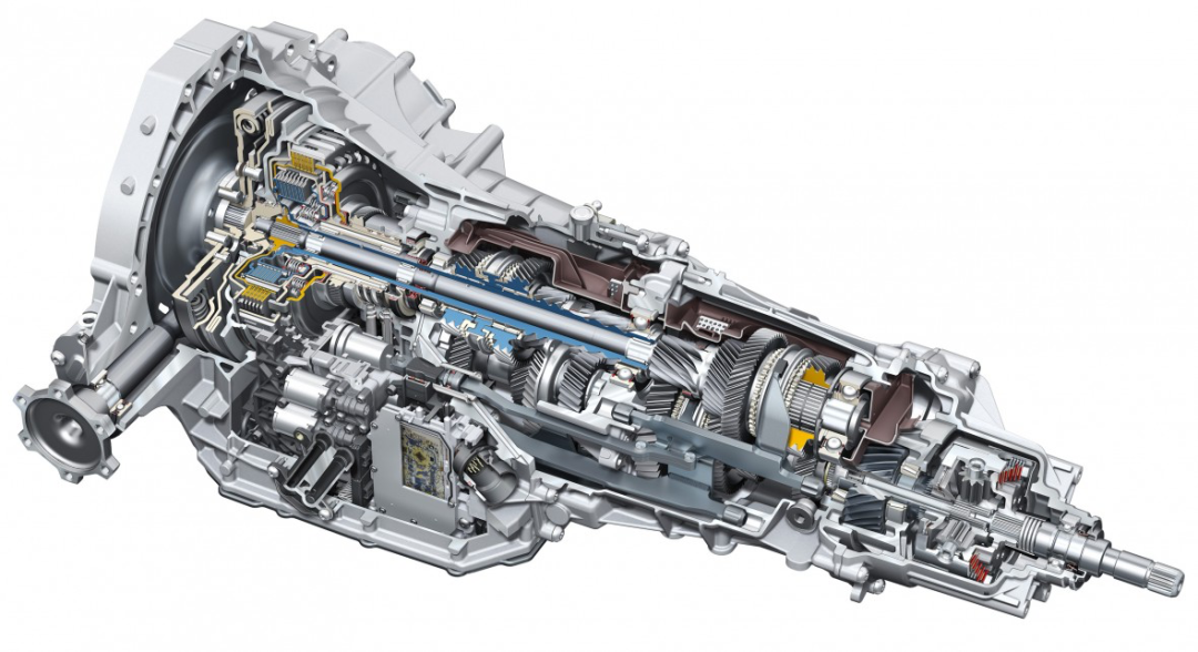
官方宣传物料
官方宣传物料
S-Tronic 的最大作用就是快;还在用 2 挡加速时,3 挡已经提前“准备好”了;在深踩油门超车时,动力几乎没有延迟,加速感非常连贯。(因为拉力赛你也看到了,一般是不刹车的)
内部非常酷
内部非常酷
另外也可以叫他们的大类名字序列式变速箱(Sequential Gearbox)
什么是偏时点火?
我们在看电影的时候,里面在右手边有很多的拉杆,这个是档把,和我们手动挡一致,但不需要踩离合,但是在变档的时候需要油门给对应的油,不然车会坏掉。
因为这里是序列式变速箱的功劳;在比赛中,除了起步,换挡通常不需要踩离合器。它配合我们下面聊过的偏时点火,能实现在全油门状态下直接“暴力”换挡而动力几乎零中断。
传统情况踩离合换挡必须松油门,涡轮压力会瞬间消失,换完挡再踩油门需要重新等增压(迟滞);有了偏时配合换挡的一瞬间,ECU执行偏时点火。虽然动力暂时切断以保护变速箱齿轮,但排气管里的爆炸维持了涡轮转速。换挡结束时,涡轮依然满压,动力衔接像电车一样顺滑。
偏时点火系统(Anti-Lag System,简称 ALS,俗称“回火”或“Bang-Bang系统”)是一种通过在排气管内产生爆炸来消除涡轮迟滞的技术。
在普通的涡轮增压车上,当驾驶员松开油门,发动机排气量骤减,驱动涡轮旋转的动力不足,导致涡轮转速下降。但是你再次踩下油门时,需要等待涡轮重新提速,这就是“迟滞”。
偏时点火的做法是:收油不关火当赛车手松开油门进入弯道时,ECU(电脑)依然控制供油系统继续喷油,但推迟点火时间;大部分汽油混合气不经过气缸燃烧,而是直接排入极高温度的排气歧管中自燃爆发;这种爆炸产生的强大气流会持续推动涡轮转子高速旋转,使涡轮在收油期间依然维持高增压状态;这个过程伴随着极响的“砰、砰”类似鞭炮或开枪的声音。虽然它能让车动力随叫随到,但代价巨大: 排气管内的高温爆炸对涡轮叶片、排气头段和气门有极强的破坏性。赛车往往每个赛段就要更换涡轮;收油时还在疯狂喷油,油耗极高。(赛车上面用是 105 油,25 元一升)
刹不住怎么行?
Brembo来了!
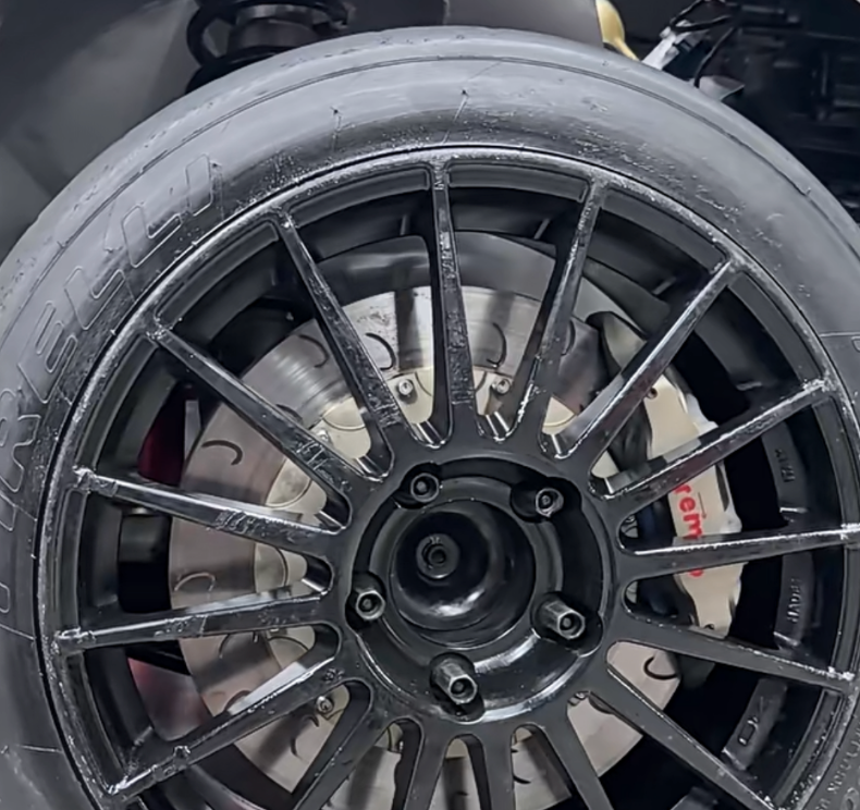
一个 15 万,一套 60 万
一个 15 万,一套 60 万
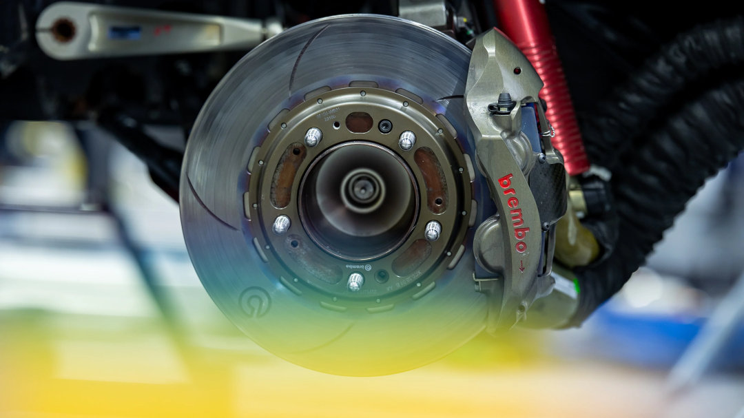
image-20260226190032399
还记得之前张弛没刹住吗?现在当然可以刹住了:
无需多言
无需多言
动力学套件的名字我忘了是什么。。。
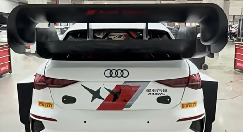
需要单独开模
需要单独开模
扩散器(Diffuser)是安装在赛车底部后端的核心套件,其主要作用是通过加速车底气流来产生下压力(Downforce),从而显著提升车辆在高速过弯时的抓地力和稳定性。
扩散器的设计利用了流体力学中的文丘里效应(Venturi Effect)和伯努利原理(Bernoulli's Principle):扩散器内部呈逐渐扩大的斜面设计。当气流从狭窄的车底进入宽大的扩散器时,气流会加速并导致压力下降;车底形成的这个“负压区”会像吸盘一样将赛车“吸”在路面上;扩散器还能让车底的高速气流在排出时平稳地减速并恢复到大气压力,减少车尾产生的紊流和阻力。
然后这个座位是 OMP 的:
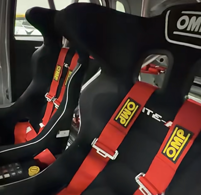
保护狗命第一名
保护狗命第一名

一坐,这就呼应上了!
一坐,这就呼应上了!
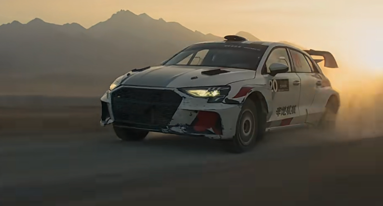
A3 的壳子,爆改的核心
A3 的壳子,爆改的核心
小结一下
听说有什么老板钱多的不知道咋花,那来这边花点,不就五百万吗?轻松花掉。
开始传统手艺(建模EPS系统)
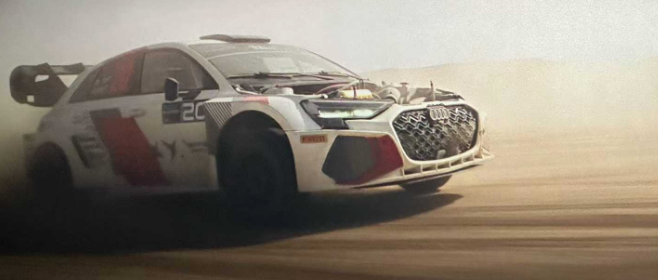
🤣,这次千里奔袭就是开的 A5:
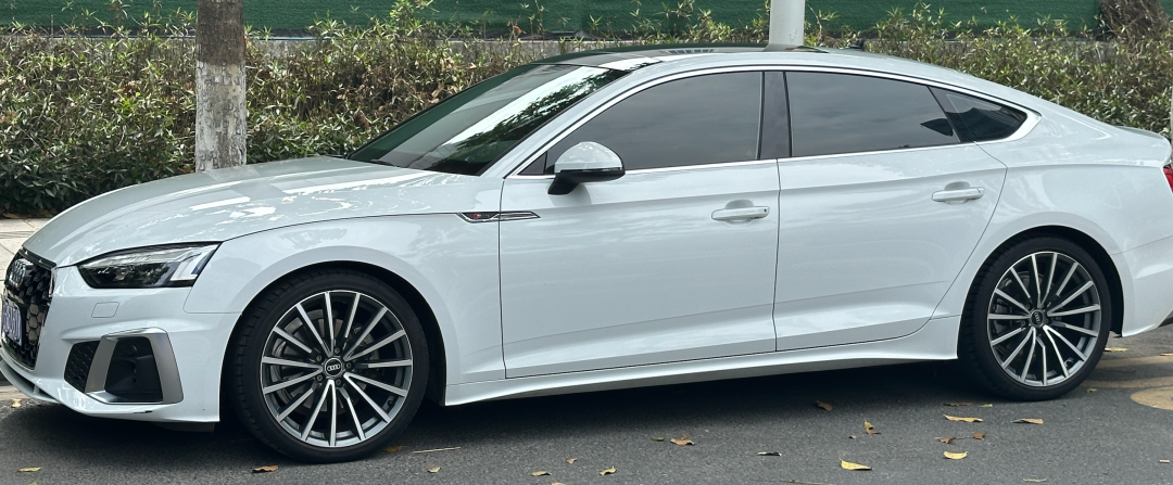
奥迪一半钱肯定是设计师拿走了,另外这个车型是轿跑版
奥迪一半钱肯定是设计师拿走了,另外这个车型是轿跑版
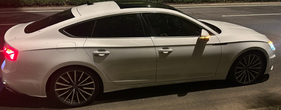
夜晚这个前脸更好看
夜晚这个前脸更好看
就是开的时间感觉坐地板上了。。。油门稍微用力,整个车都在很积极的呼应。(每次看她都得拍一张)
在电影里面的 AI 做了什么?除了一些屌屌的语音控制,我觉得其实是高级的ESP(Electronic Stability Program 电子稳定程序),也就是帮助稳定车身的一套系统,至于这个动力分配系统。
ESP 解决的不是“刹不刹得住”,而是:车还听不听你方向盘的话;典型场景:湿滑路面,高速变道,弯中给油,甩尾 / 推头。在这复杂的路况里面当然合适;它融合了多传感器信息:方向盘角度,车速,各轮轮速,横摆角速度(Yaw rate),横向加速度然后做一件事:比较“你想让车怎么走” vs “车实际怎么走”。
(小声 bb,我晚上还大致看了一本讲相关的教材,我只能说拉完了,洋洋洒洒一百页还在讲控制论,还不开始建模,等啥呢?)
ESP的闭环结构
ESP 本质上是一个多输入、多输出(MIMO)的实时姿态稳定控制系统(也可以说:以“横摆角速度”为核心状态变量的车辆姿态闭环控制系统);它控制的不是“刹车”,而是 车辆的运动状态是否符合驾驶员意图。
ESP 的被控对象是什么?
被控对象(Plant)-整车 + 轮胎 + 路面;这是一个:强非线性,参数时变,路面不确定的典型“噩梦级对象”;所以ESP 不可能做精确模型,只能做 鲁棒控制。
ESP 的状态变量
ESP 至少关心这几类状态:
驾驶员期望输入(参考信号)
方向盘转角θ
方向盘转角速度 θ
车速
这些共同定义了:“理想横摆角速度”
车辆实际状态(反馈量)
来自传感器:
横摆角速度
横向加速度
四轮轮速
关键误差信号(Error)
ESP 的核心误差不是位置,而是:
这就是闭环控制的“误差信号”
其实ESP 内部有一个“理想车辆模型,通常是:单轨模型(Bicycle Model),用来小侧偏角假设。
用于计算:
其中:
v:车速
L:轴距
δ:前轮转角(由方向盘换算)
这一步的物理含义是:“如果轮胎完全抓地,驾驶员这把方向盘,车应该怎么转”
控制目标
不是让误差为 0,而是:快速压制失控趋势,不让驾驶员察觉明显“抢方向”,可以看作这是一个 受约束的稳定控制问题。
控制手段(执行器)
ESP 不能直接控制方向盘,只能:
执行器 1:单轮制动(最核心)
左前 / 右前 / 左后 / 右后,可以完全独立控制
执行器 2:发动机扭矩限制
减小驱动力,防止继续失稳
为什么“单轮制动”能控制方向?
这是 ESP 最漂亮的一点;举例(过度转向,甩尾):
车尾向右甩,ESP 判断:
于是刹外侧前轮,产生一个反向横摆力矩
数学上可以理解为:
直接“拧回去”。
ESP 为什么不能“预测”,只能“抑制”?
因为:轮胎摩擦系数 μ 不可测,路面状态随机变化,ESP 没有未来信息
所以它的策略是:
一旦偏离参考模型,就立刻施加反向力矩
(非常棒,大致就是这样,但是鄙人觉得有点粗糙,可以再精细一点);因为控制论里面有很多的建模方式,现在这种状态方程应该是最方便的。
ESP 写成状态空间模型
用线性单轨(bicycle)模型描述车辆横向动力学,并把 ESP 的作用等效为一个可控的“附加横摆力矩” (真实车上来自“单轮制动”产生的力矩)。
模型:线性单轨 + 状态空间
选状态:
:质心横向速度
:横摆角速度(yaw rate)
输入:驾驶员转向 (前轮转角),ESP 施加的附加横摆力矩
线性轮胎侧偏力(小侧偏角):
车辆横向/横摆方程:
这可以写成标准状态空间:
用“参考横摆率”闭环
核心误差:
简单可用的参考(“理想无侧偏/低侧偏”近似):
控制律(PD):
并加饱和(代表制动能力/附着极限)。
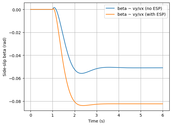
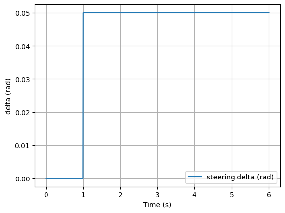
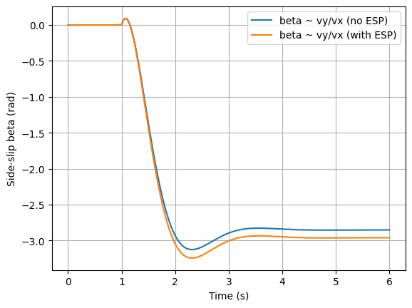
Python 仿真
- 无 ESP:只靠车辆自身横向动力学
- 有 ESP:加入 闭环抑制失稳趋势
并画出:
yaw rate
side-slip 近似
ESP 输出
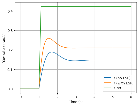
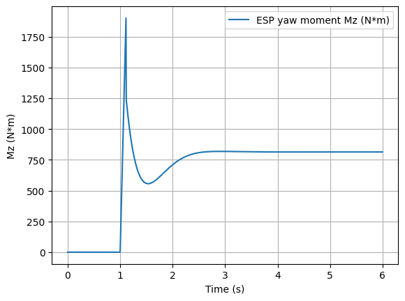
以上是一个比较不好的路面情况:
路面附着:mu_scale
1.0:干地
0.4:湿滑
0.2:冰雪
车速:vx,高速更容易触发失稳趋势
- 方向盘打多少:
delta_step - ESP 能力上限:
Mz_max,这非常接近“制动系统/轮胎摩擦”极限约束的效果 - 控制器增益:
Kp, Kd增益太大:反应猛、可能“抖” 增益太小:救不住
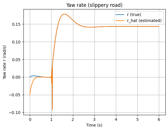
这是模拟冰雪,方向盘最剧烈的时候
这是模拟冰雪,方向盘最剧烈的时候
我们要让模型更像真实 ESP,下一步把: 变成 四个轮的制动力
并用几何关系生成横摆力矩:
(t 是轮距,符号由左右轮决定),也能加入更多可以算法来改善这个模型;这次加入侧偏角 的观测(observer) + 用 LQR 做 ESP 的 控制。
车辆模型:线性单轨(bicycle),状态
观测量(传感器能拿到的):横摆角速度 、横向加速度
来自 yaw-rate gyro
来自加速度计
观测器:Luenberger(也可以把它换成 Kalman)
控制器:LQR 计算 (等效“单轮制动产生的附加横摆力矩”)
侧偏角输出:(由估计的 得到)
LQR gain K (u = -K x_hat): [[ -89.15315449 2466.23833163]]
Observer gain L: [[-18.68235294  -5.21176471]
 [  6.17805348  -0.15482353]]
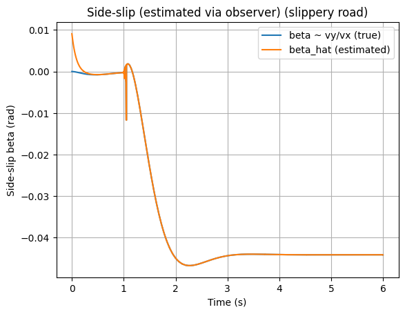
估计的 会很快贴近真实 (因为直接测了 ),估计的 会在 1~2 秒内收敛;Mz 会在转向阶跃后介入,并受到饱和限制(这对应现实里“制动能力/附着极限”)。
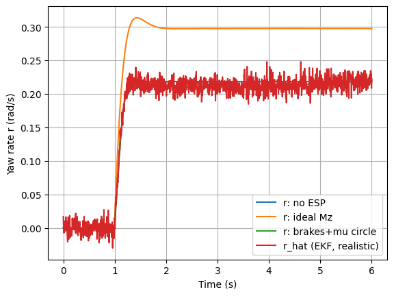
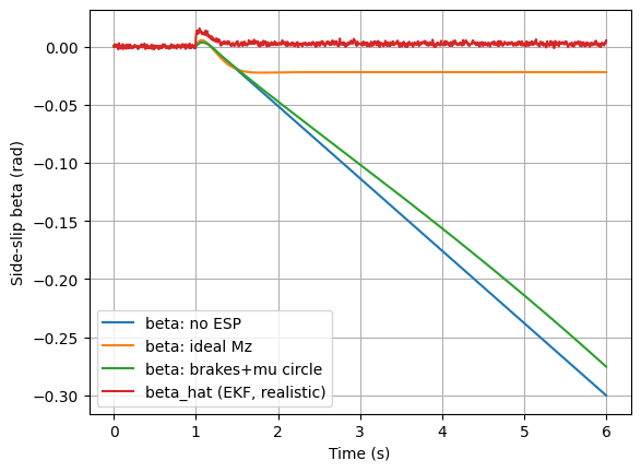
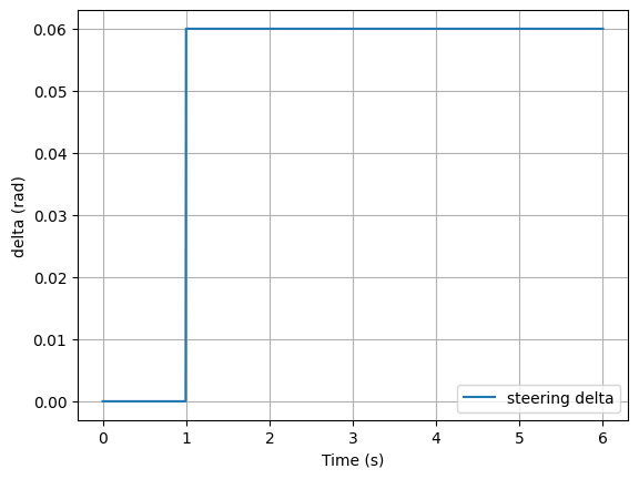
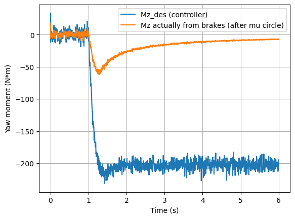
迎来最后的建模
上面的模型还是比较粗糙,最后来个完整版的,完成这篇文章,包含:
- Kalman(严格说是 EKF 框架)+ 传感器噪声:用 (横摆角速度)和 (横向加速度)做状态估计,输出 。
- 把 还原成四轮制动分配:由目标横摆力矩 分配到左右侧车轮的制动力(可进一步按前后轴分配)。
- 加入摩擦圆/轮胎饱和(救不住边界):每个轮胎满足 ,制动力越大,可用的侧向力越少,从而出现“怎么救都救不回”的极限工况。
模型内包含了Kalman(EKF框架)、四轮分配、摩擦圆饱和;简化了三点(后续建模继续加):横向载荷转移(左右轮 Fz 不同)现在只做了纵向转移(刹车前移载);更真实的轮胎模型,现在是“线性侧偏 + 摩擦圆裁剪”,还没用 Pacejka;现在看到的是“ESP 上层”,没有加入 ABS 的轮速闭环。
(太多的公式大家不爱看,看看图就好了)
(下次电影就应该让我搞点东西做展示,AI 要做数据分析,而不是一个画面,切换四轮的动力系统,咋算出来了,要🧐)
在上图可以看到:
理想 Mz:控制器想要多少 就给多少,效果通常“很漂亮”。
真实四轮 + 摩擦圆:当你为了造 去加大制动力 时,会挤占轮胎余量,使可用的 被迫缩小,出现:yaw rate 降下来了,但侧偏角/横向轨迹未必跟着变好,甚至可能更糟;这就是现实里“救车有边界”的根源。
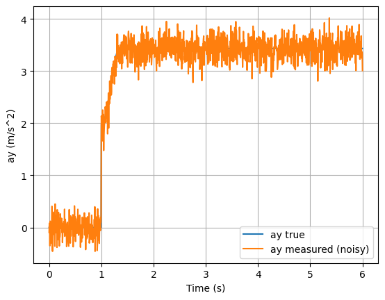
EKF 的意义
会看到 很快贴近(因为直接测),而 逐步收敛,从而给出 ;这就是“ESP 需要估计侧偏角/横向状态”的工程动机。
后记
电影很好看
电影很好看
现在国内但凡拍的像个人,票房就不会扑街。。。车是内燃机最浪漫的产物,电子,机械,动力,工程学等等学科交互的地方,每一次点火都是一次最原始能量的释放,每一次转弯都是工程学在闪烁。
可能我的模型对大多数人来讲太远,但是如果用到 RC 小车上呢?自己的小机器人上呢?或者是数学建模比赛呢?这些都是后话,总之内燃机的轰鸣,带来的不止是动力,也有可能是技术的脉动~
代码
import numpy as np
from dataclasses import dataclass
from scipy.integrate import solve_ivp
import matplotlib.pyplot as plt
# -----------------------------
# 1) Vehicle model parameters
# -----------------------------
@dataclass
class VehicleParams:
m: float = 1400.0 # kg
Iz: float = 2500.0 # kg*m^2
a: float = 1.1 # m CG -> front axle
b: float = 1.5 # m CG -> rear axle
Cf: float = 80000.0 # N/rad (front cornering stiffness)
Cr: float = 90000.0 # N/rad (rear cornering stiffness)
vx: float = 20.0 # m/s (constant longitudinal speed)
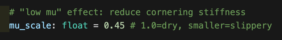
# "low mu" effect: reduce cornering stiffness
mu_scale: float = 0.45 # 1.0=dry, smaller=slippery
@property
def L(self):
return self.a + self.b
def state_space_matrices(p: VehicleParams):
"""
Linear bicycle model with states x=[vy, r]^T
Inputs: delta (steering), Mz (additional yaw moment from ESP)
"""
m, Iz, a, b, vx = p.m, p.Iz, p.a, p.b, p.vx
Cf = p.Cf * p.mu_scale
Cr = p.Cr * p.mu_scale
# A matrix components (standard linear bicycle model)
A11 = -(Cf + Cr) / (m * vx)
A12 = -vx - (a*Cf - b*Cr) / (m * vx)
A21 = -(a*Cf - b*Cr) / (Iz * vx)
A22 = -(a*a*Cf + b*b*Cr) / (Iz * vx)
A = np.array([[A11, A12],
[A21, A22]])
# steering input
B_delta = np.array([[Cf / m],
[a*Cf / Iz]])
# yaw moment input
B_M = np.array([[0.0],
[1.0 / Iz]])
return A, B_delta, B_M
# -----------------------------
# 2) Driver steering profile
# -----------------------------
def steering_delta(t, delta_step=0.05, t0=1.0):
"""
Step steering input (rad). 0.05 rad ~ 2.86 deg
"""
return delta_step if t >= t0 else 0.0
# -----------------------------
# 3) ESP controller (yaw-rate feedback)
# -----------------------------
@dataclass
class ESPGains:
Kp: float = 3500.0 # N*m per (rad/s)
Kd: float = 500.0 # N*m per (rad/s)
Mz_max: float = 2500.0 # N*m saturation (represents brake capability)
def esp_control(t, x, p: VehicleParams, g: ESPGains):
"""
Compute additional yaw moment Mz.
x = [vy, r]
"""
vy, r = x
delta = steering_delta(t)
# simple reference yaw rate
r_ref = (p.vx / p.L) * delta
e = r_ref - r
Mz = g.Kp * e - g.Kd * r
# saturation
Mz = np.clip(Mz, -g.Mz_max, g.Mz_max)
return Mz, r_ref
# -----------------------------
# 4) ODE definitions
# -----------------------------
def ode_no_esp(t, x, p: VehicleParams):
A, B_delta, B_M = state_space_matrices(p)
delta = steering_delta(t)
dx = (A @ x.reshape(-1, 1) + B_delta * delta).flatten()
return dx
def ode_with_esp(t, x, p: VehicleParams, g: ESPGains, log):
A, B_delta, B_M = state_space_matrices(p)
delta = steering_delta(t)
Mz, r_ref = esp_control(t, x, p, g)
dx = (A @ x.reshape(-1, 1) + B_delta * delta + B_M * Mz).flatten()
# logging
log["t"].append(t)
log["delta"].append(delta)
log["Mz"].append(Mz)
log["r_ref"].append(r_ref)
log["vy"].append(x[0])
log["r"].append(x[1])
return dx
# -----------------------------
# 5) Run simulation
# -----------------------------
def run():
# try a "slippery road"
p = VehicleParams(vx=22.0, mu_scale=0.35) # lower mu => harder to control
g = ESPGains(Kp=4500.0, Kd=700.0, Mz_max=2800.0)
t_span = (0.0, 6.0)
t_eval = np.linspace(t_span[0], t_span[1], 1200)
x0 = np.array([0.0, 0.0]) # start straight
# Case 1: no ESP
sol1 = solve_ivp(lambda t, x: ode_no_esp(t, x, p),
t_span, x0, t_eval=t_eval, rtol=1e-7, atol=1e-9)
# Case 2: with ESP (log everything)
log = {"t": [], "delta": [], "Mz": [], "r_ref": [], "vy": [], "r": []}
sol2 = solve_ivp(lambda t, x: ode_with_esp(t, x, p, g, log),
t_span, x0, t_eval=t_eval, rtol=1e-7, atol=1e-9)
# postprocess
vy1, r1 = sol1.y[0], sol1.y[1]
vy2, r2 = sol2.y[0], sol2.y[1]
beta1 = vy1 / p.vx
beta2 = vy2 / p.vx
# For controller logs, resample to t_eval roughly (simple interpolation)
tlog = np.array(log["t"])
Mzlog = np.array(log["Mz"])
rreflog = np.array(log["r_ref"])
# interpolation to t_eval
Mz_i = np.interp(t_eval, tlog, Mzlog)
rref_i = np.interp(t_eval, tlog, rreflog)
delta_i = np.array([steering_delta(t) for t in t_eval])
# -----------------------------
# 6) Plot
# -----------------------------
plt.figure()
plt.plot(t_eval, r1, label="r (no ESP)")
plt.plot(t_eval, r2, label="r (with ESP)")
plt.plot(t_eval, rref_i, label="r_ref")
plt.xlabel("Time (s)")
plt.ylabel("Yaw rate r (rad/s)")
plt.legend()
plt.grid(True)
plt.figure()
plt.plot(t_eval, beta1, label="beta ~ vy/vx (no ESP)")
plt.plot(t_eval, beta2, label="beta ~ vy/vx (with ESP)")
plt.xlabel("Time (s)")
plt.ylabel("Side-slip beta (rad)")
plt.legend()
plt.grid(True)
plt.figure()
plt.plot(t_eval, delta_i, label="steering delta (rad)")
plt.xlabel("Time (s)")
plt.ylabel("delta (rad)")
plt.legend()
plt.grid(True)
plt.figure()
plt.plot(t_eval, Mz_i, label="ESP yaw moment Mz (N*m)")
plt.xlabel("Time (s)")
plt.ylabel("Mz (N*m)")
plt.legend()
plt.grid(True)
plt.show()
if __name__ == "__main__":
run()
import numpy as np
from dataclasses import dataclass
from scipy.integrate import solve_ivp
from scipy.linalg import solve_continuous_are
from scipy.signal import cont2discrete
import matplotlib.pyplot as plt

# =========================
# 1) Parameters
# =========================
@dataclass
class VehicleParams:
    m: float = 1400.0         # kg
    Iz: float = 2500.0        # kg*m^2
    a: float = 1.1            # m  CG->front axle
    b: float = 1.5            # m  CG->rear axle
    track: float = 1.55       # m  track width
    h: float = 0.55           # m  CG height (for load transfer)
    vx: float = 22.0          # m/s constant longitudinal speed
    Cf: float = 80000.0       # N/rad (linear cornering stiffness)
    Cr: float = 90000.0       # N/rad
    mu: float = 0.35          # friction coefficient (slippery)
    g: float = 9.81

    @property
    def L(self) -> float:
        return self.a + self.b

@dataclass
class ControlParams:
    # LQR on estimated state xhat=[vy, r] -> u = Mz_des
    q_vy: float = 2.0
    q_r: float = 60.0
    r_u: float = 3e-6
    Mz_max: float = 2800.0        # N*m "controller desire" saturation

    # brake allocation
    front_bias: float = 0.6       # portion of side brake force on front axle
    max_brake_per_wheel: float = 6000.0  # N (cap by brake system)

@dataclass
class SensorParams:
    # measurement noise (1-sigma)
    sigma_r: float = 0.01         # rad/s
    sigma_ay: float = 0.2         # m/s^2

@dataclass
class EKFParams:
    dt: float = 0.005
    # process noise covariance (tune)
    q_vy: float = 0.5
    q_r: float = 0.5
    # initial covariance
    p0_vy: float = 1.0
    p0_r: float = 0.2

# =========================
# 2) Driver steering profile
# =========================
def steering_delta(t, step=0.06, t0=1.0):
    # 0.06 rad ~ 3.4 deg
    return step if t >= t0 else 0.0

# =========================
# 3) Linear bicycle matrices (for LQR + EKF linearization)
# =========================
def bicycle_mats(p: VehicleParams):
    m, Iz, a, b, vx = p.m, p.Iz, p.a, p.b, p.vx
    Cf, Cr = p.Cf, p.Cr

    A11 = -(Cf + Cr) / (m * vx)
    A12 = -vx - (a*Cf - b*Cr) / (m * vx)
    A21 = -(a*Cf - b*Cr) / (Iz * vx)
    A22 = -(a*a*Cf + b*b*Cr) / (Iz * vx)

    A = np.array([[A11, A12],
                  [A21, A22]])

    B_delta = np.array([[Cf / m],
                        [a*Cf / Iz]])

    # "ideal" yaw moment input
    B_M = np.array([[0.0],
                    [1.0 / Iz]])

    # measurement y = [r, ay]
    # ay = d(vy)/dt + vx*r
    C_ay = A[0, :] + np.array([0.0, vx])
    D_ay_delta = B_delta[0, 0]

    C = np.array([
        [0.0, 1.0],
        C_ay
    ])
    D = np.array([
        [0.0],
        [D_ay_delta]
    ])
    return A, B_delta, B_M, C, D

def lqr_gain(A, B, Q, R):
    P = solve_continuous_are(A, B, Q, R)
    K = np.linalg.solve(R, B.T @ P)
    return K

# =========================
# 4) Nonlinear-ish tire: friction circle saturation
# =========================
def normal_loads(p: VehicleParams, ax: float):
    """
    Simple longitudinal load transfer only.
    ax: longitudinal acceleration (negative for braking)
    """
    m, g, h, L = p.m, p.g, p.h, p.L
    a, b = p.a, p.b

    Fz_front_static = m*g*(b/L)
    Fz_rear_static  = m*g*(a/L)

    dFz = m*ax*h/L  # braking ax<0 -> dFz<0 -> front load increases by -dFz
    Fz_front = Fz_front_static - dFz
    Fz_rear  = Fz_rear_static + dFz

    # per wheel (left/right split, no lateral transfer in this simple model)
    return (Fz_front/2, Fz_front/2, Fz_rear/2, Fz_rear/2)  # FL, FR, RL, RR

def lateral_forces_linear(p: VehicleParams, vy: float, r: float, delta: float):
    """
    Axle lateral forces from linear bicycle model:
    returns Fy_front_total, Fy_rear_total
    """
    vx = p.vx
    a, b = p.a, p.b
    Cf, Cr = p.Cf, p.Cr

    alpha_f = delta - (vy + a*r)/vx
    alpha_r = -(vy - b*r)/vx

    Fy_f = Cf * alpha_f
    Fy_r = Cr * alpha_r
    return Fy_f, Fy_r

def apply_friction_circle(Fx, Fy, muFz):
    """
    Saturate (Fx, Fy) so that sqrt(Fx^2 + Fy^2) <= muFz
    Keep direction as much as possible (scale if needed).
    """
    mag = np.sqrt(Fx*Fx + Fy*Fy)
    if mag <= muFz or muFz <= 0:
        return Fx, Fy
    scale = muFz / (mag + 1e-12)
    return Fx*scale, Fy*scale

# =========================
# 5) Brake allocation: Mz_des -> four wheel brake forces Fx_i (negative)
# =========================
def allocate_brakes_from_Mz(p: VehicleParams, c: ControlParams, Mz_des: float):
    """
    Use side braking to generate yaw moment:
    Mz = sum(y_i * Fx_i), y_left=+t/2, y_right=-t/2, Fx_i negative for braking.
    To get positive Mz, brake RIGHT side (y=-t/2, Fx<0 => Mz positive).

    Allocation:
      - choose one side based on sign(Mz_des)
      - split to front/rear by front_bias
      - per-wheel cap
    Return Fx_FL, Fx_FR, Fx_RL, Fx_RR (negative for braking)
    """
    t = p.track
    if abs(Mz_des) < 1e-6:
        return 0.0, 0.0, 0.0, 0.0

    # choose side
    brake_right = (Mz_des > 0.0)
    y = -t/2 if brake_right else +t/2  # y of that side wheels

    # need sum Fx_side such that Mz_des = y * sumFx_side
    sumFx_side = Mz_des / (y + 1e-12)  # should be negative (braking)
    # enforce braking direction (negative)
    sumFx_side = min(sumFx_side, 0.0)

    Fx_front = c.front_bias * sumFx_side
    Fx_rear  = (1.0 - c.front_bias) * sumFx_side

    # per-wheel
    Fx_front_each = np.clip(Fx_front, -2*c.max_brake_per_wheel, 0.0) / 2.0
    Fx_rear_each  = np.clip(Fx_rear,  -2*c.max_brake_per_wheel, 0.0) / 2.0

    Fx_FL = Fx_FR = Fx_RL = Fx_RR = 0.0
    if brake_right:
        Fx_FR = Fx_front_each
        Fx_RR = Fx_rear_each
    else:
        Fx_FL = Fx_front_each
        Fx_RL = Fx_rear_each

    return Fx_FL, Fx_FR, Fx_RL, Fx_RR

# =========================
# 6) Plant dynamics (with friction circle + brake allocation)
# =========================
def plant_step(p: VehicleParams, vy: float, r: float, delta: float, Fx_wheels):
    """
    One-step continuous dynamics:
      - compute linear axle Fy
      - split axle Fy to left/right equally
      - apply friction circle per wheel with Fx_i and mu*Fz_i
      - sum wheel forces -> dynamics
    Return (dvy, dr), and also ay, Fx_total, Fy_total, Mz_from_brakes
    """
    m, Iz, vx, a, b = p.m, p.Iz, p.vx, p.a, p.b

    Fx_FL, Fx_FR, Fx_RL, Fx_RR = Fx_wheels
    Fx_total = Fx_FL + Fx_FR + Fx_RL + Fx_RR

    # approximate ax from total Fx
    ax = Fx_total / m

    # normal loads with longitudinal transfer
    Fz_FL, Fz_FR, Fz_RL, Fz_RR = normal_loads(p, ax)
    mu = p.mu

    # linear axle lateral forces
    Fy_f, Fy_r = lateral_forces_linear(p, vy, r, delta)

    # split to wheels
    Fy_FL = Fy_f / 2.0
    Fy_FR = Fy_f / 2.0
    Fy_RL = Fy_r / 2.0
    Fy_RR = Fy_r / 2.0

    # friction circle per wheel
    Fx_FL_s, Fy_FL_s = apply_friction_circle(Fx_FL, Fy_FL, mu*Fz_FL)
    Fx_FR_s, Fy_FR_s = apply_friction_circle(Fx_FR, Fy_FR, mu*Fz_FR)
    Fx_RL_s, Fy_RL_s = apply_friction_circle(Fx_RL, Fy_RL, mu*Fz_RL)
    Fx_RR_s, Fy_RR_s = apply_friction_circle(Fx_RR, Fy_RR, mu*Fz_RR)

    Fx_total_s = Fx_FL_s + Fx_FR_s + Fx_RL_s + Fx_RR_s
    Fy_total_s = Fy_FL_s + Fy_FR_s + Fy_RL_s + Fy_RR_s

    # yaw moment from lateral forces (bicycle approximation) + from longitudinal brake asymmetry
    # Mz_lat = a*Fy_f - b*Fy_r (use saturated sums per axle)
    Fy_f_s = Fy_FL_s + Fy_FR_s
    Fy_r_s = Fy_RL_s + Fy_RR_s
    Mz_lat = a*Fy_f_s - b*Fy_r_s

    # Mz_brake = sum(y_i * Fx_i)
    t = p.track
    yL, yR = +t/2.0, -t/2.0
    Mz_brake = yL*(Fx_FL_s + Fx_RL_s) + yR*(Fx_FR_s + Fx_RR_s)

    # dynamics
    dvy = (Fy_total_s / m) - vx*r
    dr  = (Mz_lat + Mz_brake) / Iz

    # ay = dvy + vx*r
    ay = dvy + vx*r

    return dvy, dr, ay, Fx_total_s, Fy_total_s, Mz_brake

# =========================
# 7) EKF (discrete-time) using linearized model for prediction
# =========================
class SimpleEKF:
    """
    State: x=[vy, r]
    Measure: y=[r, ay]
    Prediction uses discretized linear bicycle model:
      x_{k+1} = Ad x_k + Bd_delta delta_k + Bd_M * Mz_ideal_k  (for ideal case)
    In our "realistic" case, we still use same linear model as a filter model.
    """
    def __init__(self, p: VehicleParams, s: SensorParams, ekf: EKFParams):
        self.p = p
        self.s = s
        self.ekf = ekf

        A, B_delta, B_M, C, D = bicycle_mats(p)
        self.A = A
        self.Bd = B_delta
        self.Bm = B_M
        self.C = C
        self.D = D

        # discretize (ZOH) with dt
        dt = ekf.dt
        Ad, Bd, _, _, _ = cont2discrete((A, np.hstack([B_delta, B_M]), C, np.zeros((2,2))), dt)

        self.Ad = Ad
        self.Bd2 = Bd  # columns: [delta, Mz]

        # covariances
        self.Q = np.diag([ekf.q_vy, ekf.q_r]) * dt
        self.R = np.diag([s.sigma_r**2, s.sigma_ay**2])

        self.x = np.array([0.0, 0.0])
        self.P = np.diag([ekf.p0_vy, ekf.p0_r])

    def predict(self, delta, Mz_model):
        u = np.array([delta, Mz_model])
        self.x = (self.Ad @ self.x) + (self.Bd2 @ u)
        self.P = self.Ad @ self.P @ self.Ad.T + self.Q

    def update(self, y_meas, delta, Mz_model):
        """
        y = C x + D*delta + noise, but note ay depends also on dynamics.
        We'll keep measurement model:
          y_hat = C x + D*delta
        (This is approximate but works as a minimal EKF-like filter.)
        """
        y_hat = (self.C @ self.x) + (self.D.flatten() * delta)
        # innovation
        innov = y_meas - y_hat

        S = self.C @ self.P @ self.C.T + self.R
        K = self.P @ self.C.T @ np.linalg.inv(S)
        self.x = self.x + K @ innov
        self.P = (np.eye(2) - K @ self.C) @ self.P

# =========================
# 8) Simulation harness
# =========================
def run_sim():
    p = VehicleParams(vx=22.0, mu=0.35)
    c = ControlParams()
    s = SensorParams()
    ekf_cfg = EKFParams(dt=0.005)

    # LQR (ideal yaw-moment controller): u = Mz_des = -K xhat
    A, B_delta, B_M, C, D = bicycle_mats(p)
    Q = np.diag([c.q_vy, c.q_r])
    R = np.array([[c.r_u]])
    K = lqr_gain(A, B_M, Q, R)  # 1x2

    # EKF
    filt = SimpleEKF(p, s, ekf_cfg)

    # time grid
    T = 6.0
    dt = ekf_cfg.dt
    N = int(T/dt) + 1
    ts = np.linspace(0.0, T, N)

    # ---------
    # three modes:
    # (1) no ESP (Fx_wheels=0)
    # (2) ideal ESP: apply "Mz_des" directly as external yaw moment (not realistic)
    # (3) realistic ESP: allocate to brakes + friction circle
    # ---------
    def simulate_mode(mode: int):
        vy, r = 0.0, 0.0
        filt.x[:] = np.array([0.2, -0.05])   # initial mismatch to show convergence
        filt.P[:] = np.diag([ekf_cfg.p0_vy, ekf_cfg.p0_r])

        logs = {
            "t": [], "delta": [],
            "vy": [], "r": [], "beta": [],
            "vy_hat": [], "r_hat": [], "beta_hat": [],
            "ay_meas": [], "ay_true": [],
            "Mz_des": [], "Mz_brake": [],
            "Fx_total": [], "Fy_total": [],
            "Fx_FL": [], "Fx_FR": [], "Fx_RL": [], "Fx_RR": []
        }

        for t in ts:
            delta = steering_delta(t)

            # controller uses estimated state
            xhat = filt.x.copy()
            Mz_des = float(-(K @ xhat.reshape(-1,1)).item())
            Mz_des = float(np.clip(Mz_des, -c.Mz_max, c.Mz_max))

            if mode == 1:
                # no ESP
                Fx_wheels = (0.0, 0.0, 0.0, 0.0)
                dvy, dr, ay_true, Fx_total, Fy_total, Mz_br = plant_step(p, vy, r, delta, Fx_wheels)

            elif mode == 2:
                # ideal Mz directly injected: emulate by converting to equivalent asymmetric Fx on track with no saturation
                # We'll implement as: compute dr = (Mz_lat + Mz_des)/Iz, i.e., bypass brake allocation and friction limit.
                # Use linear axle Fy (no friction circle) for this mode.
                Fy_f, Fy_r = lateral_forces_linear(p, vy, r, delta)
                dvy = (Fy_f + Fy_r)/p.m - p.vx*r
                dr  = (p.a*Fy_f - p.b*Fy_r + Mz_des)/p.Iz
                ay_true = dvy + p.vx*r
                Fx_total, Fy_total, Mz_br = 0.0, (Fy_f+Fy_r), Mz_des
                Fx_wheels = (0.0, 0.0, 0.0, 0.0)

            else:
                # realistic: allocate to brakes + friction circle
                Fx_wheels = allocate_brakes_from_Mz(p, c, Mz_des)
                dvy, dr, ay_true, Fx_total, Fy_total, Mz_br = plant_step(p, vy, r, delta, Fx_wheels)

            # integrate (Euler; small dt)
            vy += dvy * dt
            r  += dr  * dt

            # measurement with noise: y=[r, ay]
            y_meas = np.array([
                r + np.random.randn()*s.sigma_r,
                ay_true + np.random.randn()*s.sigma_ay
            ])

            # filter predict/update (model uses Mz_des as "Mz_model")
            filt.predict(delta, Mz_des)
            filt.update(y_meas, delta, Mz_des)

            # logs
            logs["t"].append(t)
            logs["delta"].append(delta)
            logs["vy"].append(vy)
            logs["r"].append(r)
            logs["beta"].append(vy/p.vx)

            logs["vy_hat"].append(filt.x[0])
            logs["r_hat"].append(filt.x[1])
            logs["beta_hat"].append(filt.x[0]/p.vx)

            logs["ay_meas"].append(y_meas[1])
            logs["ay_true"].append(ay_true)

            logs["Mz_des"].append(Mz_des)
            logs["Mz_brake"].append(Mz_br)

            logs["Fx_total"].append(Fx_total)
            logs["Fy_total"].append(Fy_total)

            Fx_FL, Fx_FR, Fx_RL, Fx_RR = Fx_wheels
            logs["Fx_FL"].append(Fx_FL)
            logs["Fx_FR"].append(Fx_FR)
            logs["Fx_RL"].append(Fx_RL)
            logs["Fx_RR"].append(Fx_RR)

        for k in logs:
            logs[k] = np.array(logs[k])
        return logs

    np.random.seed(7)  # reproducible
    log_no   = simulate_mode(1)
    np.random.seed(7)
    log_ideal= simulate_mode(2)
    np.random.seed(7)
    log_real = simulate_mode(3)

    # =========================
    # 9) Plot
    # =========================
    t = log_real["t"]

    plt.figure()
    plt.plot(t, log_no["r"], label="r: no ESP")
    plt.plot(t, log_ideal["r"], label="r: ideal Mz")
    plt.plot(t, log_real["r"], label="r: brakes+mu circle")
    plt.plot(t, log_real["r_hat"], label="r_hat (EKF, realistic)")
    plt.xlabel("Time (s)")
    plt.ylabel("Yaw rate r (rad/s)")
    plt.grid(True)
    plt.legend()

    plt.figure()
    plt.plot(t, log_no["beta"], label="beta: no ESP")
    plt.plot(t, log_ideal["beta"], label="beta: ideal Mz")
    plt.plot(t, log_real["beta"], label="beta: brakes+mu circle")
    plt.plot(t, log_real["beta_hat"], label="beta_hat (EKF, realistic)")
    plt.xlabel("Time (s)")
    plt.ylabel("Side-slip beta (rad)")
    plt.grid(True)
    plt.legend()

    plt.figure()
    plt.plot(t, log_real["delta"], label="steering delta")
    plt.xlabel("Time (s)")
    plt.ylabel("delta (rad)")
    plt.grid(True)
    plt.legend()

    plt.figure()
    plt.plot(t, log_ideal["Mz_des"], label="Mz_des (controller)")
    plt.plot(t, log_real["Mz_brake"], label="Mz actually from brakes (after mu circle)")
    plt.xlabel("Time (s)")
    plt.ylabel("Yaw moment (N*m)")
    plt.grid(True)
    plt.legend()

    plt.figure()
    plt.plot(t, log_real["Fx_FR"], label="Fx_FR")
    plt.plot(t, log_real["Fx_RR"], label="Fx_RR")
    plt.plot(t, log_real["Fx_FL"], label="Fx_FL")
    plt.plot(t, log_real["Fx_RL"], label="Fx_RL")
    plt.xlabel("Time (s)")
    plt.ylabel("Wheel longitudinal force Fx (N, negative=brake)")
    plt.grid(True)
    plt.legend()

    plt.figure()
    plt.plot(t, log_real["ay_true"], label="ay true")
    plt.plot(t, log_real["ay_meas"], label="ay measured (noisy)")
    plt.xlabel("Time (s)")
    plt.ylabel("ay (m/s^2)")
    plt.grid(True)
    plt.legend()

    plt.show()

if __name__ == "__main__":
    run_sim()
本文参与 腾讯云自媒体同步曝光计划,分享自微信公众号。
原始发表:2026-02-26,如有侵权请联系 cloudcommunity@tencent.com 删除
评论
登录后参与评论
推荐阅读
目录
腾讯云开发者

Copyright © 2013 - 2026 Tencent Cloud. All Rights Reserved. 腾讯云 版权所有
深圳市腾讯计算机系统有限公司 ICP备案/许可证号:粤B2-20090059 ![]() 粤公网安备44030502008569号
粤公网安备44030502008569号
腾讯云计算(北京)有限责任公司 京ICP证150476号 | 京ICP备11018762号