R:用于聚类树状图的ggplot高度调整

Question

其思想是将R包、ClustOfVar和ggdendro结合起来，对变量聚类进行可视化总结。

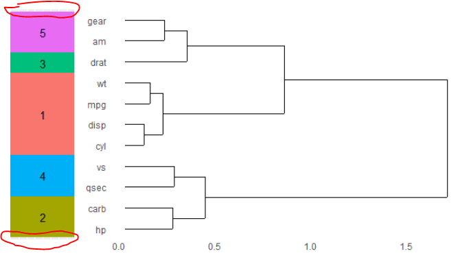
当数据中没有列时，结果非常好，只是有些区域没有覆盖(如下图所示)。例如，使用mtcars：

library(plyr)
library(ggplot2)
library(gtable)
library(grid)
library(gridExtra)

library(ClustOfVar)
library(ggdendro)

fit = hclustvar(X.quanti = mtcars)

labels = cutree(fit,k = 5)

labelx = data.frame(Names=names(labels),group = paste("Group",as.vector(labels)),num=as.vector(labels))

p1 = ggdendrogram(as.dendrogram(fit), rotate=TRUE)

df2<-data.frame(cluster=cutree(fit, k =5), states=factor(fit$labels,levels=fit$labels[fit$order]))
df3<-ddply(df2,.(cluster),summarise,pos=mean(as.numeric(states)))

p2 = ggplot(df2,aes(states,y=1,fill=factor(cluster)))+geom_tile()+
  scale_y_continuous(expand=c(0,0))+
  theme(axis.title=element_blank(),
        axis.ticks=element_blank(),
        axis.text=element_blank(),
        legend.position="none")+coord_flip()+
  geom_text(data=df3,aes(x=pos,label=cluster))
gp1<-ggplotGrob(p1)
gp2<-ggplotGrob(p2)  
maxHeight = grid::unit.pmax(gp1$heights[2:5], gp2$heights[2:5])
gp1$heights[2:5] <- as.list(maxHeight)
gp2$heights[2:5] <- as.list(maxHeight)
grid.arrange(gp2, gp1, ncol=2,widths=c(1/6,5/6))

​

​

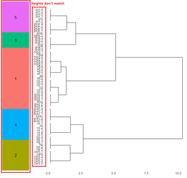
当有大量列时，会出现另一个问题。也就是说，彩色瓷砖部分的高度与树状图的高度不匹配。

library(ClustOfVar)
library(ggdendro)
X = data.frame(mtcars,mtcars,mtcars,mtcars,mtcars,mtcars)

fit = hclustvar(X.quanti = X)

labels = cutree(fit,k = 5)

labelx = data.frame(Names=names(labels),group = paste("Group",as.vector(labels)),num=as.vector(labels))

p1 = ggdendrogram(as.dendrogram(fit), rotate=TRUE)

df2<-data.frame(cluster=cutree(fit, k =5), states=factor(fit$labels,levels=fit$labels[fit$order]))
df3<-ddply(df2,.(cluster),summarise,pos=mean(as.numeric(states)))

p2 = ggplot(df2,aes(states,y=1,fill=factor(cluster)))+geom_tile()+
  scale_y_continuous(expand=c(0,0))+
  theme(axis.title=element_blank(),
        axis.ticks=element_blank(),
        axis.text=element_blank(),
        legend.position="none")+coord_flip()+
  geom_text(data=df3,aes(x=pos,label=cluster))
gp1<-ggplotGrob(p1)
gp2<-ggplotGrob(p2)  
maxHeight = grid::unit.pmax(gp1$heights[2:5], gp2$heights[2:5])
gp1$heights[2:5] <- as.list(maxHeight)
gp2$heights[2:5] <- as.list(maxHeight)
grid.arrange(gp2, gp1, ncol=2,widths=c(1/6,5/6))

​

​

@Sandy实际上为这个提供了一个很好的解决方案，如果我们将R升级到3.3.1版。R: ggplot slight adjustment for clustering summary

但是，由于我不能更改部署在公司服务器中的R版本，我想知道是否还有其他解决办法可以对齐这两个部分。

Answer 1

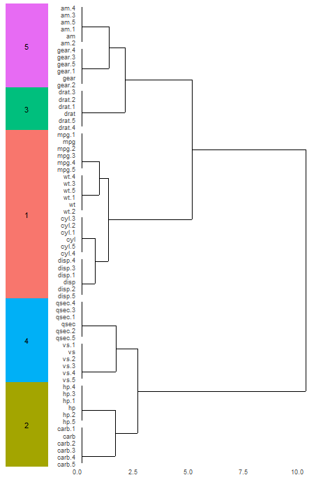
据我所知，你的代码并没有错。问题是，当您合并这两个图时，您正在尝试将连续的尺度与离散的尺度相匹配。而且，ggdendrogram()似乎为y轴增加了额外的空间.

library(plyr)
library(ggplot2)
library(gtable)
library(grid)
library(gridExtra)

library(ClustOfVar)
library(ggdendro)

# Data
X = data.frame(mtcars,mtcars,mtcars,mtcars,mtcars,mtcars)

# Cluster analysis
fit = hclustvar(X.quanti = X)

# Labels data frames
df2 <- data.frame(cluster = cutree(fit, k =5), 
     states = factor(fit$labels, levels = fit$labels[fit$order]))
df3 <- ddply(df2, .(cluster), summarise, pos = mean(as.numeric(states)))

# Dendrogram
# scale_x_continuous() for p1 should match scale_x_discrete() from p2
# scale_x_continuous strips off the labels. I grab them from df2
# scale _y_continuous() puts a little space between the labels and the dendrogram
p1 <- ggdendrogram(as.dendrogram(fit), rotate = TRUE) +
     scale_x_continuous(expand = c(0, 0.5), labels = levels(df2$states), breaks = 1:length(df2$states)) +
     scale_y_continuous(expand = c(0.02, 0)) 

# Tiles and labels
p2 <- ggplot(df2,aes(states, y = 1, fill = factor(cluster))) +
  geom_tile() +
  scale_y_continuous(expand = c(0, 0)) + 
  scale_x_discrete(expand = c(0, 0)) +
  geom_text(data = df3, aes(x = pos, label = cluster)) +
  coord_flip() +
  theme(axis.title = element_blank(),
        axis.ticks = element_blank(),
        axis.text = element_blank(),
        legend.position = "none")

# Get the ggplot grobs
gp1 <- ggplotGrob(p1)
gp2 <- ggplotGrob(p2)  

# Make sure the heights match
maxHeight <- unit.pmax(gp1$heights, gp2$heights)
gp1$heights <- as.list(maxHeight)
gp2$heights <- as.list(maxHeight)

# Combine the two plots
grid.arrange(gp2, gp1, ncol = 2,widths = c(1/6, 5/6))

​

​