python中离散傅里叶变换(FT)的技巧和香蕉皮

Question

在python中进行傅里叶变换时，我对有用的技巧和香蕉皮感兴趣。

请给介绍代码示例进入这个主题，以及更多的建议在高级主题，如：频率滤波器，连续FT，高维FT。

Answer 1

从python (Numpy)中的二维离散Fourier变换开始：

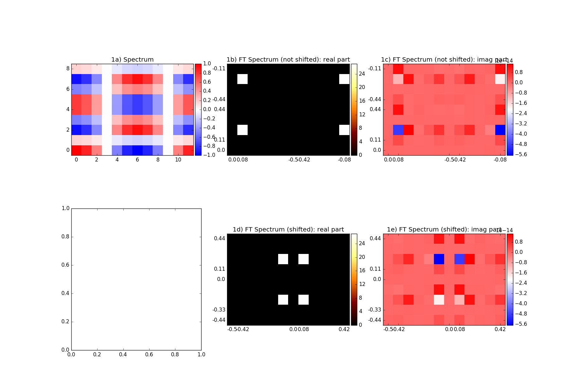
1.频率排序

我们应该注意numpy.fft库对频率的排序。fft例程首先是零，然后是正频率，然后是负频率(图1b，1c)。函数fftshift可以用于按预期建立顺序，即从负值到正值，需要fftshift例程(图1d，1e)。

代码示例：

import matplotlib.pyplot as plt
import numpy as np
from mpl_toolkits.axes_grid1 import make_axes_locatable

fig, ((ax1,ax2,ax3),(ax4,ax5,ax6)) = plt.subplots(2,3, figsize=(18.3,12.5))


#Spectrum and FT
spec=np.ndarray(shape=(12,9))
for ii in range(0,spec.shape[0]):
    for jj in range(0,spec.shape[1]):
        spec[ii,jj]=np.cos(2*np.pi*ii/spec.shape[0])*np.cos(4*np.pi*jj/spec.shape[1])
        
spec_ft = np.fft.fft2(spec)
spec_ftShifted = np.fft.fftshift(np.fft.fft2(spec))
   
#Frequencies / labels axes
xFreq=np.around(np.fft.fftfreq(spec.shape[0]),decimals=2)
yFreq=np.around(np.fft.fftfreq(spec.shape[1]),decimals=2)
xFreqShifted=np.around(np.fft.fftshift(np.fft.fftfreq(spec.shape[0])),decimals=2)
yFreqShifted=np.around(np.fft.fftshift(np.fft.fftfreq(spec.shape[1])),decimals=2)


#Plotting
ax=ax1
ax.set_title('1a) Spectrum')
im=ax.imshow(spec.T,origin='lower',cmap='bwr',interpolation='none')
divider0 = make_axes_locatable(ax)
cax=divider0.append_axes("right", size="5%", pad=0.05)
cbar=plt.colorbar(im,cax=cax)
#
ax=ax2
ax.set_title('1b) FT Spectrum (not shifted): real part')
im=ax.imshow(spec_ft.real.T,origin='lower',cmap='afmhot',interpolation='none')
ax.set_xticks([0,1,int(spec.shape[0]/2),int(spec.shape[0]/2+1),spec.shape[0]-1])
ax.set_xticklabels([xFreq[0],xFreq[1],xFreq[int(spec.shape[0]/2)],xFreq[int(spec.shape[0]/2+1)],xFreq[spec.shape[0]-1]])
ax.set_yticks([0,1,int(spec.shape[1]/2),int(spec.shape[1]/2+1),spec.shape[1]-1])
ax.set_yticklabels([yFreq[0],yFreq[1],yFreq[int(spec.shape[1]/2)],yFreq[int(spec.shape[1]/2+1)],yFreq[spec.shape[1]-1]])
divider0 = make_axes_locatable(ax)
cax=divider0.append_axes("right", size="5%", pad=0.05)
cbar=plt.colorbar(im,cax=cax)
#
ax=ax3
ax.set_title('1c) FT Spectrum (not shifted): imag part')
im=ax.imshow(spec_ft.imag.T,origin='lower',cmap='bwr',interpolation='none')
ax.set_xticks([0,1,int(spec.shape[0]/2),int(spec.shape[0]/2+1),spec.shape[0]-1])
ax.set_xticklabels([xFreq[0],xFreq[1],xFreq[int(spec.shape[0]/2)],xFreq[int(spec.shape[0]/2+1)],xFreq[spec.shape[0]-1]])
ax.set_yticks([0,1,int(spec.shape[1]/2),int(spec.shape[1]/2+1),spec.shape[1]-1])
ax.set_yticklabels([yFreq[0],yFreq[1],yFreq[int(spec.shape[1]/2)],yFreq[int(spec.shape[1]/2+1)],yFreq[spec.shape[1]-1]])
divider0 = make_axes_locatable(ax)
cax=divider0.append_axes("right", size="5%", pad=0.05)
cbar=plt.colorbar(im,cax=cax)
#
ax=ax5
ax.set_title('1d) FT Spectrum (shifted): real part')
im=ax.imshow(spec_ftShifted.real.T,origin='lower',cmap='afmhot',interpolation='none')
ax.set_xticks([0,1,int(spec.shape[0]/2),int(spec.shape[0]/2+1),spec.shape[0]-1])
ax.set_xticklabels([xFreqShifted[0],xFreqShifted[1],xFreqShifted[int(spec.shape[0]/2)],xFreqShifted[int(spec.shape[0]/2+1)],xFreqShifted[spec.shape[0]-1]])
ax.set_yticks([0,1,int(spec.shape[1]/2),int(spec.shape[1]/2+1),spec.shape[1]-1])
ax.set_yticklabels([yFreqShifted[0],yFreqShifted[1],yFreqShifted[int(spec.shape[1]/2)],yFreqShifted[int(spec.shape[1]/2+1)],yFreqShifted[spec.shape[1]-1]])
divider0 = make_axes_locatable(ax)
cax=divider0.append_axes("right", size="5%", pad=0.05)
cbar=plt.colorbar(im,cax=cax)
#
ax=ax6
ax.set_title('1e) FT Spectrum (shifted): imag part')
im=ax.imshow(spec_ftShifted.imag.T,origin='lower',cmap='bwr',interpolation='none')
ax.set_xticks([0,1,int(spec.shape[0]/2),int(spec.shape[0]/2+1),spec.shape[0]-1])
ax.set_xticklabels([xFreqShifted[0],xFreqShifted[1],xFreqShifted[int(spec.shape[0]/2)],xFreqShifted[int(spec.shape[0]/2+1)],xFreqShifted[spec.shape[0]-1]])
ax.set_yticks([0,1,int(spec.shape[1]/2),int(spec.shape[1]/2+1),spec.shape[1]-1])
ax.set_yticklabels([yFreqShifted[0],yFreqShifted[1],yFreqShifted[int(spec.shape[1]/2)],yFreqShifted[int(spec.shape[1]/2+1)],yFreqShifted[spec.shape[1]-1]])
divider0 = make_axes_locatable(ax)
cax=divider0.append_axes("right", size="5%", pad=0.05)
cbar=plt.colorbar(im,cax=cax)

plt.show()

输出：

​

​

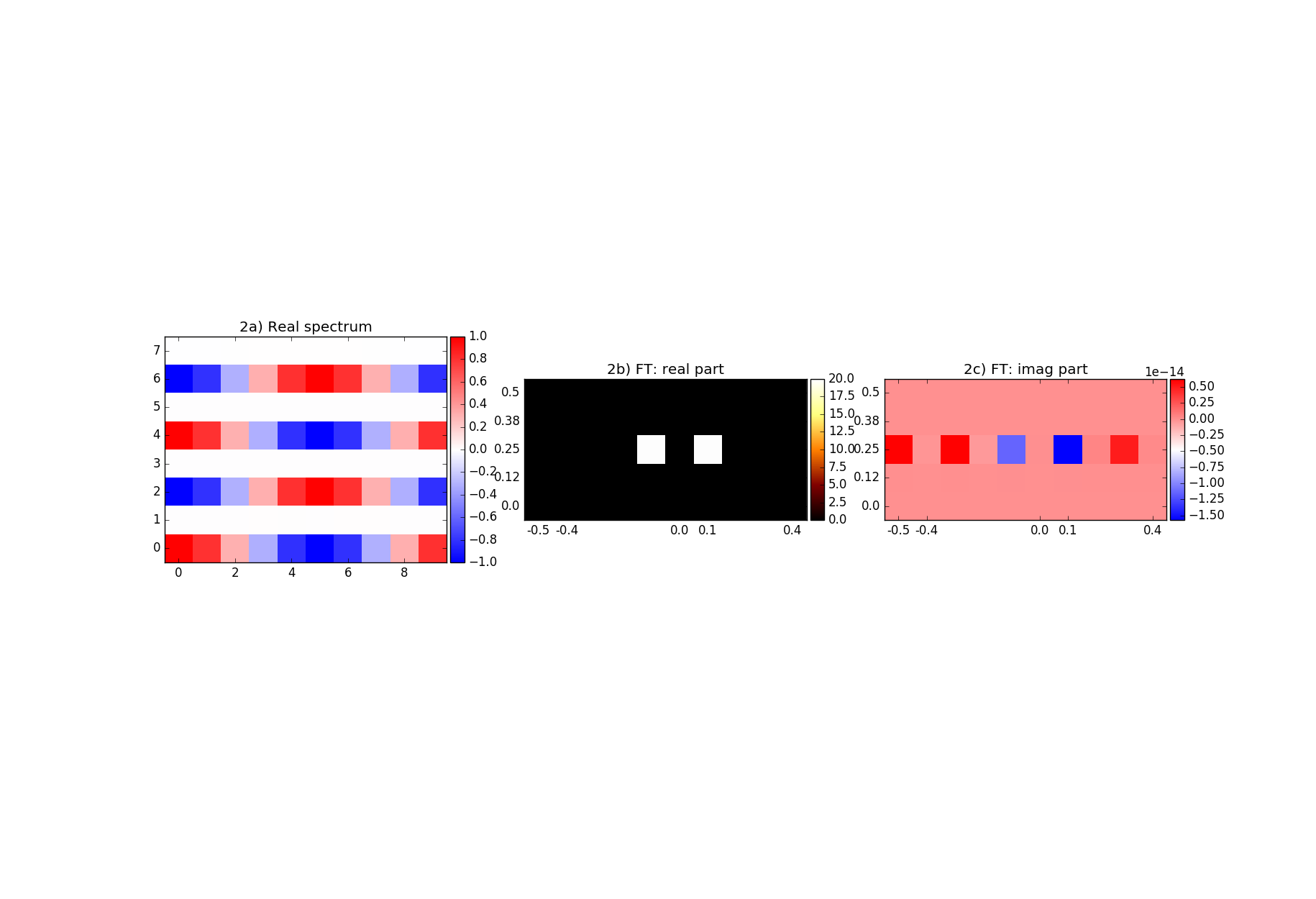
2.实值FFT

实际值输入阵列(rfft)的FT利用了这样一个事实，即FT必须是hermitian。函数F为hermitian，当: F(f)=F(-f)*

因此，只需要存储一半大小的数组。小心：，我们将在3.中看到，当使用rfft时，有一些香蕉皮。

代码示例：

import matplotlib.pyplot as plt
import numpy as np
from mpl_toolkits.axes_grid1 import make_axes_locatable

fig, ((ax1,ax2,ax3)) = plt.subplots(1,3, figsize=(18.3,12.5))


#Spectrum and FT
spec=np.ndarray(shape=(10,8))
for ii in range(0,spec.shape[0]):
    for jj in range(0,spec.shape[1]):
        spec[ii,jj]=np.cos(2*np.pi*ii/spec.shape[0])*np.cos(4*np.pi*jj/spec.shape[1])
        #spec[ii,jj]=(-1)**(ii+jj)
        #spec[:,jj]=np.cos(2*np.pi*jj/spec.shape[1])
        #spec[ii,:]=np.cos(2*np.pi*ii/spec.shape[0])
        
spec_ft=np.fft.fftshift(np.fft.rfft2(spec),axes=0)

#Frequencies / labels axes
xFreq=np.around(np.fft.fftshift(np.fft.fftfreq(spec.shape[0])),decimals=2)
yFreq=np.around(np.fft.rfftfreq(spec.shape[1]),decimals=2)


#Plotting   
ax=ax1
ax.set_title('2a) Real spectrum')
im=ax.imshow(spec.T,origin='lower',cmap='bwr',interpolation='none')
divider0 = make_axes_locatable(ax)
cax=divider0.append_axes("right", size="5%", pad=0.05)
cbar=plt.colorbar(im,cax=cax)
#
ax=ax2
ax.set_title('2b) FT: real part')
im=ax.imshow(spec_ft.real.T,origin='lower',cmap='afmhot',interpolation='none')
ax.set_xticks([0,1,int(len(xFreq)/2),int(len(xFreq)/2+1),len(xFreq)-1])
ax.set_xticklabels([xFreq[0],xFreq[1],xFreq[int(len(xFreq)/2)],xFreq[int(len(xFreq)/2+1)],xFreq[len(xFreq)-1]])
ax.set_yticks([0,1,int(len(yFreq)/2),int(len(yFreq)/2+1),len(yFreq)-1])
ax.set_yticklabels([yFreq[0],yFreq[1],yFreq[int(len(yFreq)/2)],yFreq[int(len(yFreq)/2+1)],yFreq[len(yFreq)-1]])
divider0 = make_axes_locatable(ax)
cax=divider0.append_axes("right", size="5%", pad=0.05)
cbar=plt.colorbar(im,cax=cax)
#
ax3.set_title('2c) FT: imag part')
im3=ax3.imshow(spec_ft.imag.T,origin='lower',cmap='bwr',interpolation='none')
ax3.set_xticks([0,1,int(len(xFreq)/2),int(len(xFreq)/2+1),len(xFreq)-1])
ax3.set_xticklabels([xFreq[0],xFreq[1],xFreq[int(len(xFreq)/2)],xFreq[int(len(xFreq)/2+1)],xFreq[len(xFreq)-1]])
ax3.set_yticks([0,1,int(len(yFreq)/2),int(len(yFreq)/2+1),len(yFreq)-1])
ax3.set_yticklabels([yFreq[0],yFreq[1],yFreq[int(len(yFreq)/2)],yFreq[int(len(yFreq)/2+1)],yFreq[len(yFreq)-1]])
divider0 = make_axes_locatable(ax3)
cax=divider0.append_axes("right", size="5%", pad=0.05)
cbar=plt.colorbar(im3,cax=cax)
    
plt.show()

输出：

​

​

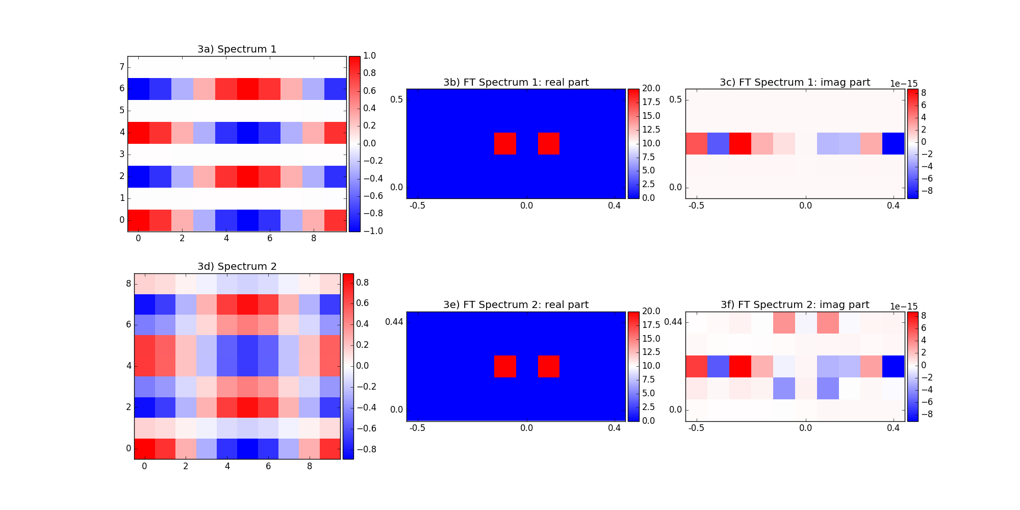
3.实值逆FFT

rfft的问题是，它不是模棱两可。这意味着，从FT ndarry的像素n_ft数来看，无法判断实际空间n_rs中的数组有多少像素。有2选项

n_rs= (n_ft-1)*2或n_rs= (n_ft-1)*2+1

图3a和3d显示了2个实际值的2d-数组。我们看到他们的FT看起来完全一样(3b，3e)。虚部(3c和3f)几乎都是0。因此，如果我们不知道它的维数/形状，那么从FT谱中我们无法得出真实的空间谱是怎样的。由于这个原因，使用标准fft而不是rfft.可能更具有普遍性。

警告:艾夫特模棱两可！

代码示例：

import matplotlib.pyplot as plt
import numpy as np
from mpl_toolkits.axes_grid1 import make_axes_locatable

fig, ((ax1,ax2,ax3),(ax4,ax5,ax6)) = plt.subplots(2,3,figsize=(20,10))

#Spectrum and FT
#generating spectrum: this is just used to generate real spectrum option 1/2 and is not plotted
#it is equivalent to: spec_ft1 and spec_ft2
spec_ft=np.zeros(shape=(10,5))
spec_ft[4,2]=20
spec_ft[6,2]=20
#
spec_r1=np.fft.irfft2(np.fft.ifftshift(spec_ft,axes=0),s=(spec_ft.shape[0],(spec_ft.shape[1]-1)*2))
spec_r2=np.fft.irfft2(np.fft.ifftshift(spec_ft,axes=0),s=(spec_ft.shape[0],(spec_ft.shape[1]-1)*2+1))
#
spec_ft1=np.fft.fftshift(np.fft.rfft2(spec_r1),axes=0)
spec_ft2=np.fft.fftshift(np.fft.rfft2(spec_r2),axes=0)

#Frequencies / labels axes
xFreq1=np.around(np.fft.fftshift(np.fft.fftfreq(spec_r1.shape[0])),decimals=2)
yFreq1=np.around(np.fft.rfftfreq(spec_r1.shape[1]),decimals=2)
xFreq2=np.around(np.fft.fftshift(np.fft.fftfreq(spec_r2.shape[0])),decimals=2)
yFreq2=np.around(np.fft.rfftfreq(spec_r2.shape[1]),decimals=2)

#Plotting  
ax=ax1
ax.set_title('3a) Spectrum 1')
im=ax.imshow(spec_r1.real.T,origin='lower',cmap='bwr',interpolation='none')
divider0 = make_axes_locatable(ax)
cax=divider0.append_axes("right", size="5%", pad=0.05)
cbar=plt.colorbar(im,cax=cax)
#
ax=ax2
ax.set_title('3b) FT Spectrum 1: real part')
im=ax.imshow(spec_ft1.real.T,origin='lower',cmap='bwr',interpolation='none')
ax.set_xticks([0,int(len(xFreq1)/2),len(xFreq1)-1])
ax.set_xticklabels([xFreq1[0],xFreq1[int(len(xFreq1)/2)],xFreq1[-1]])
ax.set_yticks([0,len(yFreq1)-1])
ax.set_yticklabels([yFreq1[0],yFreq1[-1]])
divider0 = make_axes_locatable(ax)
cax=divider0.append_axes("right", size="5%", pad=0.05)
cbar=plt.colorbar(im,cax=cax)
#
ax=ax3
ax.set_title('3c) FT Spectrum 1: imag part')
im=ax.imshow(spec_ft1.imag.T,origin='lower',cmap='bwr',interpolation='none')
ax.set_xticks([0,int(len(xFreq1)/2),len(xFreq1)-1])
ax.set_xticklabels([xFreq1[0],xFreq1[int(len(xFreq1)/2)],xFreq1[-1]])
ax.set_yticks([0,len(yFreq1)-1])
ax.set_yticklabels([yFreq1[0],yFreq1[-1]])
divider0 = make_axes_locatable(ax)
cax=divider0.append_axes("right", size="5%", pad=0.05)
cbar=plt.colorbar(im,cax=cax)
#
ax=ax4
ax.set_title('3d) Spectrum 2')
im=ax.imshow(spec_r2.real.T,origin='lower',cmap='bwr',interpolation='none')
divider0 = make_axes_locatable(ax)
cax=divider0.append_axes("right", size="5%", pad=0.05)
cbar=plt.colorbar(im,cax=cax)
#
ax=ax5
ax.set_title('3e) FT Spectrum 2: real part')
im=ax.imshow(spec_ft2.real.T,origin='lower',cmap='bwr',interpolation='none')
ax.set_xticks([0,int(len(xFreq2)/2),len(xFreq2)-1])
ax.set_xticklabels([xFreq2[0],xFreq2[int(len(xFreq2)/2)],xFreq2[-1]])
ax.set_yticks([0,len(yFreq2)-1])
ax.set_yticklabels([yFreq2[0],yFreq2[-1]])
divider0 = make_axes_locatable(ax)
cax=divider0.append_axes("right", size="5%", pad=0.05)
cbar=plt.colorbar(im,cax=cax)
#
ax=ax6
ax.set_title('3f) FT Spectrum 2: imag part')
im=ax.imshow(spec_ft2.imag.T,origin='lower',cmap='bwr',interpolation='none')
ax.set_xticks([0,int(len(xFreq2)/2),len(xFreq2)-1])
ax.set_xticklabels([xFreq2[0],xFreq2[int(len(xFreq2)/2)],xFreq2[-1]])
ax.set_yticks([0,len(yFreq2)-1])
ax.set_yticklabels([yFreq2[0],yFreq2[-1]])
divider0 = make_axes_locatable(ax)
cax=divider0.append_axes("right", size="5%", pad=0.05)
cbar=plt.colorbar(im,cax=cax)
    
plt.show()

输出：

​

​

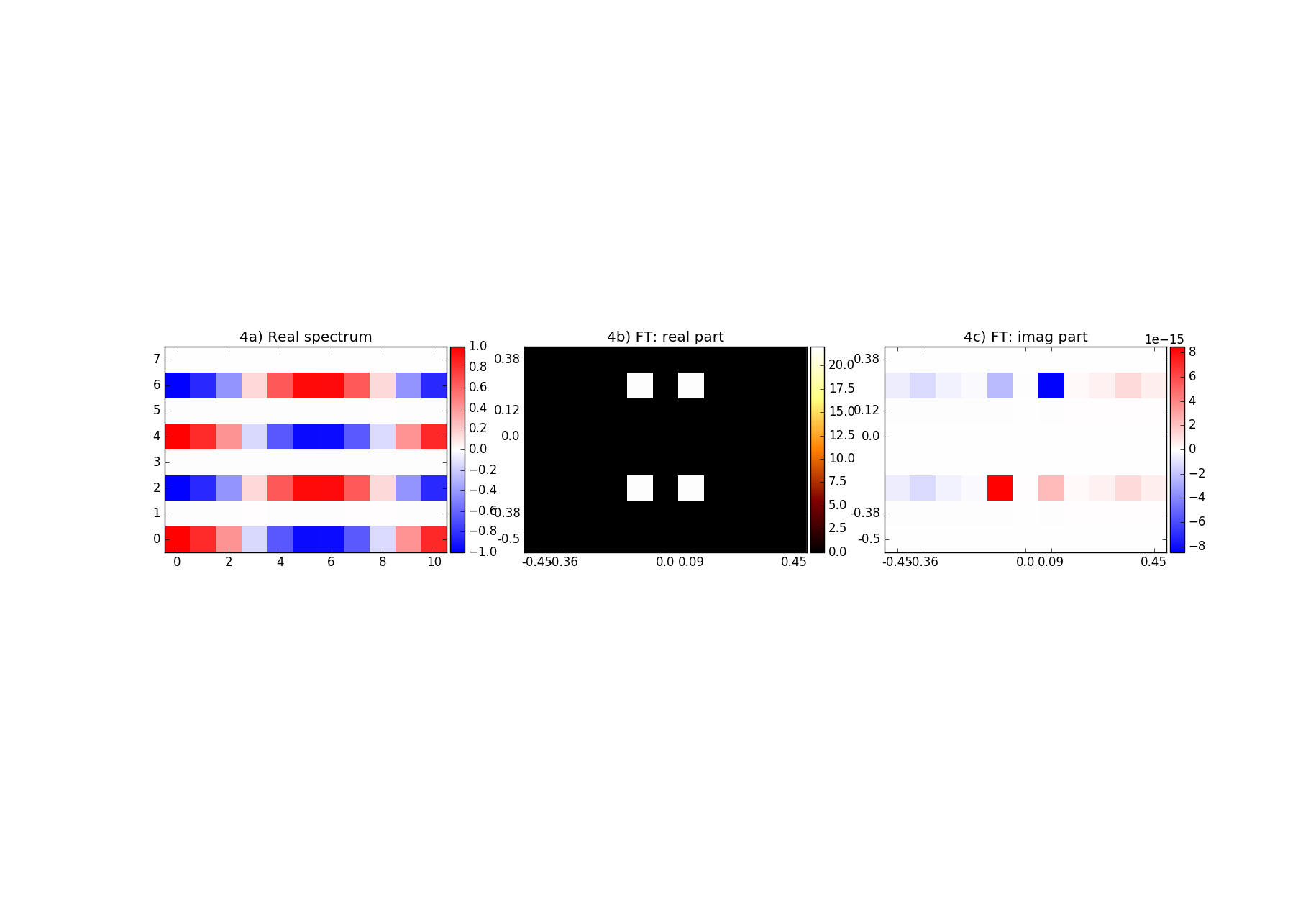
4. FFT

这里是一个例子，如何使用FT，而不包括频谱知识的真实。我们看到FT阵列的形状和实际空间阵列的形状是一样的。

代码示例：

import matplotlib.pyplot as plt
import numpy as np
from mpl_toolkits.axes_grid1 import make_axes_locatable

fig, ((ax1,ax2,ax3)) = plt.subplots(1,3, figsize=(18.3,12.5))

#Spectrum and FT
spec=np.ndarray(shape=(11,8))
for ii in range(0,spec.shape[0]):
    for jj in range(0,spec.shape[1]):
        #spec[ii,jj]=(-1)**(ii+jj)
        #spec[ii,jj]=np.sin(2*np.pi*ii/spec.shape[0])*np.sin(4*np.pi*jj/spec.shape[1])
        spec[ii,jj]=np.cos(2*np.pi*ii/spec.shape[0])*np.cos(4*np.pi*jj/spec.shape[1])
        #spec[:,jj]=np.cos(2*np.pi*jj/spec.shape[1])
        #spec[ii,:]=np.cos(2*np.pi*ii/spec.shape[0])

spec_ft=np.fft.fftshift(np.fft.fft2(spec))

#Frequencies / labels axes
xFreq=np.around(np.fft.fftshift(np.fft.fftfreq(spec.shape[0])),decimals=2)
yFreq=np.around(np.fft.fftshift(np.fft.fftfreq(spec.shape[1])),decimals=2)

#Plotting
ax=ax1
ax.set_title('4a) Real spectrum')
im=ax.imshow(spec.T,origin='lower',cmap='bwr',interpolation='none')
divider0 = make_axes_locatable(ax)
cax=divider0.append_axes("right", size="5%", pad=0.05)
cbar=plt.colorbar(im,cax=cax)
#
ax=ax2
ax.set_title('4b) FT: real part')
im=ax.imshow(spec_ft.real.T,origin='lower',cmap='afmhot',interpolation='none')
ax.set_xticks([0,1,int(len(xFreq)/2),int(len(xFreq)/2+1),len(xFreq)-1])
ax.set_xticklabels([xFreq[0],xFreq[1],xFreq[int(len(xFreq)/2)],xFreq[int(len(xFreq)/2+1)],xFreq[len(xFreq)-1]])
ax.set_yticks([0,1,int(len(yFreq)/2),int(len(yFreq)/2+1),len(yFreq)-1])
ax.set_yticklabels([yFreq[0],yFreq[1],yFreq[int(len(yFreq)/2)],yFreq[int(len(yFreq)/2+1)],yFreq[len(yFreq)-1]])
divider0 = make_axes_locatable(ax)
cax=divider0.append_axes("right", size="5%", pad=0.05)
cbar=plt.colorbar(im,cax=cax)
#
ax=ax3
ax.set_title('4c) FT: imag part')
im=ax.imshow(spec_ft.imag.T,origin='lower',cmap='bwr',interpolation='none')
ax.set_xticks([0,1,int(len(xFreq)/2),int(len(xFreq)/2+1),len(xFreq)-1])
ax.set_xticklabels([xFreq[0],xFreq[1],xFreq[int(len(xFreq)/2)],xFreq[int(len(xFreq)/2+1)],xFreq[len(xFreq)-1]])
ax.set_yticks([0,1,int(len(yFreq)/2),int(len(yFreq)/2+1),len(yFreq)-1])
ax.set_yticklabels([yFreq[0],yFreq[1],yFreq[int(len(yFreq)/2)],yFreq[int(len(yFreq)/2+1)],yFreq[len(yFreq)-1]])
divider0 = make_axes_locatable(ax)
cax=divider0.append_axes("right", size="5%", pad=0.05)
cbar=plt.colorbar(im,cax=cax)
    
plt.show()

输出：

​

​

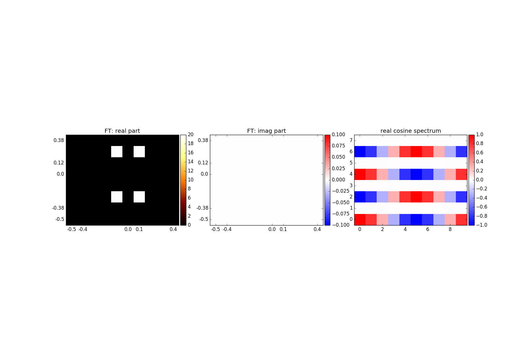
5.逆FFT

当我们进行逆FT时，实际空间ndarray将是一个复数。由于数值的精度，这些数值将有一些无穷小的小虚部。

COde示例：

import matplotlib.pyplot as plt
import numpy as np
from mpl_toolkits.axes_grid1 import make_axes_locatable

fig, ((ax1,ax2,ax3)) = plt.subplots(1,3, figsize=(18.3,12.5))

#Spectrum and FT
spec_ft=np.zeros(shape=(10,8))
spec_ft[4,2]=20
spec_ft[4,6]=20
spec_ft[6,2]=20
spec_ft[6,6]=20

spec_ift=np.fft.ifft2(np.fft.ifftshift(spec_ft))
        

#Frequencies / labels axes
xFreq=np.around(np.fft.fftshift(np.fft.fftfreq(spec_ift.shape[0])),decimals=2)
yFreq=np.around(np.fft.fftshift(np.fft.fftfreq(spec_ift.shape[1])),decimals=2)

#Plotting
ax=ax1
ax.set_title('FT: real part')
im=ax.imshow(spec_ft.real.T,origin='lower',cmap='afmhot',interpolation='none')
ax.set_xticks([0,1,int(len(xFreq)/2),int(len(xFreq)/2+1),len(xFreq)-1])
ax.set_xticklabels([xFreq[0],xFreq[1],xFreq[int(len(xFreq)/2)],xFreq[int(len(xFreq)/2+1)],xFreq[len(xFreq)-1]])
ax.set_yticks([0,1,int(len(yFreq)/2),int(len(yFreq)/2+1),len(yFreq)-1])
ax.set_yticklabels([yFreq[0],yFreq[1],yFreq[int(len(yFreq)/2)],yFreq[int(len(yFreq)/2+1)],yFreq[len(yFreq)-1]])
divider0 = make_axes_locatable(ax)
cax=divider0.append_axes("right", size="5%", pad=0.05)
cbar=plt.colorbar(im,cax=cax)
#
ax=ax2
ax.set_title('FT: imag part')
im=ax.imshow(spec_ft.imag.T,origin='lower',cmap='bwr',interpolation='none')
ax.set_xticks([0,1,int(len(xFreq)/2),int(len(xFreq)/2+1),len(xFreq)-1])
ax.set_xticklabels([xFreq[0],xFreq[1],xFreq[int(len(xFreq)/2)],xFreq[int(len(xFreq)/2+1)],xFreq[len(xFreq)-1]])
ax.set_yticks([0,1,int(len(yFreq)/2),int(len(yFreq)/2+1),len(yFreq)-1])
ax.set_yticklabels([yFreq[0],yFreq[1],yFreq[int(len(yFreq)/2)],yFreq[int(len(yFreq)/2+1)],yFreq[len(yFreq)-1]])
divider0 = make_axes_locatable(ax)
cax=divider0.append_axes("right", size="5%", pad=0.05)
cbar=plt.colorbar(im,cax=cax)
#
ax=ax3
ax.set_title('real cosine spectrum')
im=ax.imshow(spec_ift.real.T,origin='lower',cmap='bwr',interpolation='none')
divider0 = make_axes_locatable(ax)
cax=divider0.append_axes("right", size="5%", pad=0.05)
cbar=plt.colorbar(im,cax=cax)
        
plt.show()

输出：

​

​