龙格-库塔法ode45在deSolve中的自适应时间步长

Question

我希望使用来自deSolve R包的显式Runge方法ode45(别名rk45dp7)来解决具有可变步长的ODE问题。

根据deSolve文档，可以用ode45方法对rk求解器函数使用自适应或可变的时间步骤，而不是等距的时间步骤，但我不知道如何做到这一点。

rk功能是这样命名的：

rk(y, times, func, parms, rtol = 1e-6, atol = 1e-6, verbose = FALSE, tcrit = NULL,
hmin = 0, hmax = NULL, hini = hmax, ynames = TRUE, method = rkMethod("rk45dp7", ... ), 
maxsteps = 5000, dllname = NULL, initfunc = dllname, initpar = parms, rpar = NULL, 
ipar = NULL, nout = 0, outnames = NULL, forcings = NULL, initforc = NULL, fcontrol = 
NULL, events = NULL, ...)

当时间是期望y的显式估计的时间向量时。

对于距离为0.01的等距时间步长，我可以将次数写成

times <- seq(0, 100, 0.01)

假设我想要解区间从0到100的方程，我如何定义时间而不给出步长？

任何帮助都将不胜感激。

Answer 1

这里有两个问题。首先，如果要指定具有多个增量的时间向量，请使用此方法(例如)：

times <- c(seq(0,0.9,0.1),seq(1,10,1))
times
#  [1]  0.0  0.1  0.2  0.3  0.4  0.5  0.6  0.7  0.8  0.9  1.0  2.0  3.0  4.0  5.0  6.0  7.0  8.0  9.0 10.0

这里，我们有0,1乘0.1，1,10，1。

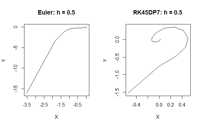
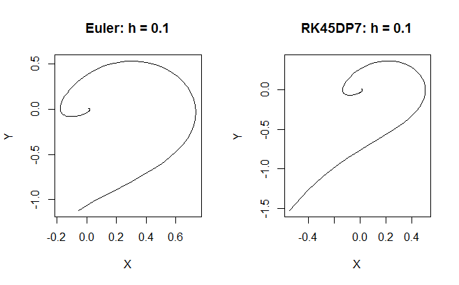
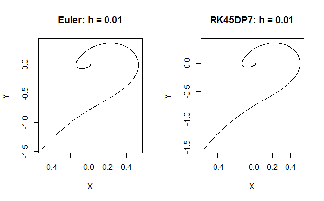
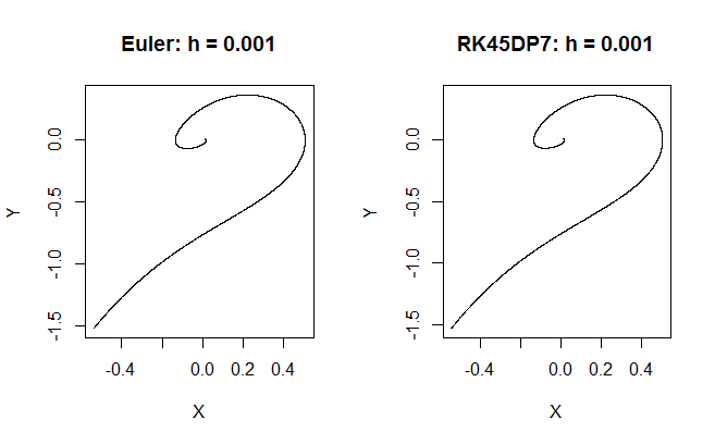
但是实际上不必这样做:参数times=告诉rk(...)报告结果的时间。自适应算法将内部调整时间增量，以便在参数指定的时间获得精确的结果。因此，对于自适应算法，例如，method="rk45dp7"，您不需要做任何事情。对于非自适应算法，例如method="euler"，该算法使用的时间增量实际上是times=中指定的增量。您可以在这个简单的例子中看到这一点的效果，它集成了Van der Pol振荡器。

y.prime <- function(t,y.vector,b) {    # Van der Pol oscillator
  x <- y.vector[1]
  y <- y.vector[2]
  x.prime <- y
  y.prime <- b*y*(1-x)^2 - x
  return(list(c(x=x.prime,y=y.prime)))
}
h  <- .001                  # time increment
t  <-  seq(0,10,h)          # times to report results
y0 <- c(0.01,0.01)          # initial conditions
euler   <- rk(y0, t,func=y.prime,parms=1,method="euler")
rk45dp7 <- rk(y0, t,func=y.prime,parms=1, method="rk45dp7")
# plot x vs. y
par(mfrow=c(1,2))
plot(euler[,2],euler[,3], type="l",xlab="X",ylab="Y",main=paste("Euler: h =",format(h,digits=3)))
plot(rk45dp7[,2],rk45dp7[,3], type="l",xlab="X",ylab="Y",main=paste("RK45DP7: h =",format(h,digits=3)))

下面是几个h值的结果的比较。注意，对于method="rk45dp7"，h < 0.5的结果是稳定的。这是因为rk45dp7正在根据需要内部调整时间增量。对于method="euler"，结果与rk45dp7不匹配，直到h~0.01。

​

​