and在模型规格和置信区间方面的意外行为

Question

我的数据是包含许多零的整数。我想用二项式广义线性模型分别对零点进行建模。在模型语句中，我在倾斜体的左侧指定了Y>0，这给了我一个二进制(TRUE，FALSE)向量。我使用emmeans包指定(type = "response")进一步分析了数据。然后，我意识到(根据我的实际数据)，信任间隔似乎消失了。我尝试解决这个问题，并决定在我的数据框架中分别创建一个包含TRUE和FALSE值的新变量。这个解决了问题。为什么会发生这种情况？

下面是再现这种行为的代码(尽管效果并不像我原来的数据集那样明显)：

require(emmeans)
# example data
d <- structure(list(X = structure(c(1L, 1L, 1L, 1L, 1L, 1L, 1L, 1L, 
1L, 1L, 2L, 2L, 2L, 2L, 2L, 2L, 2L, 2L, 2L, 2L, 3L, 3L, 3L, 3L, 
3L, 3L, 3L, 3L, 3L, 3L, 4L, 4L, 4L, 4L, 4L, 4L, 4L, 4L, 4L, 4L
), .Label = c("A", "B", "C", "D"), class = "factor"), Y = c(0L, 
4L, 4L, 5L, 6L, 5L, 6L, 7L, 8L, 9L, 0L, 0L, 3L, 4L, 1L, 5L, 2L, 
3L, 2L, 1L, 0L, 0L, 0L, 0L, 0L, 12L, 11L, 6L, 8L, 11L, 0L, 0L, 
0L, 0L, 0L, 12L, 13L, 11L, 12L, 16L)), class = "data.frame", row.names = c(NA, 
-40L))

# add additional variable - set every value > 0 to TRUE, otherwise FALSE
d$no0 <- d$Y>0 

下面是使用模型中的关系运算符>的第一个模型：

# binomial GLM using `Y>0` on the left side
m1 <- glm(Y>0 ~ X, family = binomial(), d)
summary(m1)

Call:
glm(formula = Y > 0 ~ X, family = binomial(), data = d)

Deviance Residuals: 
    Min       1Q   Median       3Q      Max  
-2.1460  -1.1774   0.4590   0.7954   1.1774  

Coefficients:
            Estimate Std. Error z value Pr(>|z|)  
(Intercept)   2.1972     1.0540   2.085   0.0371 *
XB           -0.8109     1.3175  -0.615   0.5382  
XC           -2.1972     1.2292  -1.788   0.0739 .
XD           -2.1972     1.2292  -1.788   0.0739 .
---
Signif. codes:  0 ‘***’ 0.001 ‘**’ 0.01 ‘*’ 0.05 ‘.’ 0.1 ‘ ’ 1

(Dispersion parameter for binomial family taken to be 1)

    Null deviance: 50.446  on 39  degrees of freedom
Residual deviance: 44.236  on 36  degrees of freedom
AIC: 52.236

Number of Fisher Scoring iterations: 4

下面是使用新变量的第二个模型：

# binomial GLM using variable no0
m2 <- glm(no0 ~ X, family = binomial(), d)
summary(m2)

Call:
glm(formula = no0 ~ X, family = binomial(), data = d)

Deviance Residuals: 
    Min       1Q   Median       3Q      Max  
-2.1460  -1.1774   0.4590   0.7954   1.1774  

Coefficients:
            Estimate Std. Error z value Pr(>|z|)  
(Intercept)   2.1972     1.0540   2.085   0.0371 *
XB           -0.8109     1.3175  -0.615   0.5382  
XC           -2.1972     1.2292  -1.788   0.0739 .
XD           -2.1972     1.2292  -1.788   0.0739 .
---
Signif. codes:  0 ‘***’ 0.001 ‘**’ 0.01 ‘*’ 0.05 ‘.’ 0.1 ‘ ’ 1

(Dispersion parameter for binomial family taken to be 1)

    Null deviance: 50.446  on 39  degrees of freedom
Residual deviance: 44.236  on 36  degrees of freedom
AIC: 52.236

Number of Fisher Scoring iterations: 4

到目前为止，输出是相同的。然后，我继续运行模型1和模型2的emmeans()函数，不使用-- type = "response"参数：

(em1 <- emmeans(m1, ~ X))
 X emmean    SE  df asymp.LCL asymp.UCL
 A   2.20 1.054 Inf     0.131      4.26
 B   1.39 0.791 Inf    -0.163      2.94
 C   0.00 0.632 Inf    -1.240      1.24
 D   0.00 0.632 Inf    -1.240      1.24

Results are given on the logit (not the response) scale. 
Confidence level used: 0.95 

(em2 <- emmeans(m2, ~ X))
 X emmean    SE  df asymp.LCL asymp.UCL
 A   2.20 1.054 Inf     0.131      4.26
 B   1.39 0.791 Inf    -0.163      2.94
 C   0.00 0.632 Inf    -1.240      1.24
 D   0.00 0.632 Inf    -1.240      1.24

Results are given on the logit (not the response) scale. 
Confidence level used: 0.95 

一切都很好。但是，当我添加type = response参数时，除了置信区间不同(比较下面的两个输出)外，一切看起来都很好：

(em3 <- emmeans(m1, ~ X, type = "response"))
 X response     SE  df asymp.LCL asymp.UCL
 A      0.9 0.0949 Inf     0.714      1.09
 B      0.8 0.1265 Inf     0.552      1.05
 C      0.5 0.1581 Inf     0.190      0.81
 D      0.5 0.1581 Inf     0.190      0.81

Unknown transformation ">": no transformation done 
Confidence level used: 0.95 

(em4 <- emmeans(m2, ~ X, type = "response"))
 X prob     SE  df asymp.LCL asymp.UCL
 A  0.9 0.0949 Inf     0.533     0.986
 B  0.8 0.1265 Inf     0.459     0.950
 C  0.5 0.1581 Inf     0.225     0.775
 D  0.5 0.1581 Inf     0.225     0.775

Confidence level used: 0.95 
Intervals are back-transformed from the logit scale 

我看到第一个输出(Unknown transformation ">": no transformation done)中有一个警告，但是为什么它只影响置信区间？

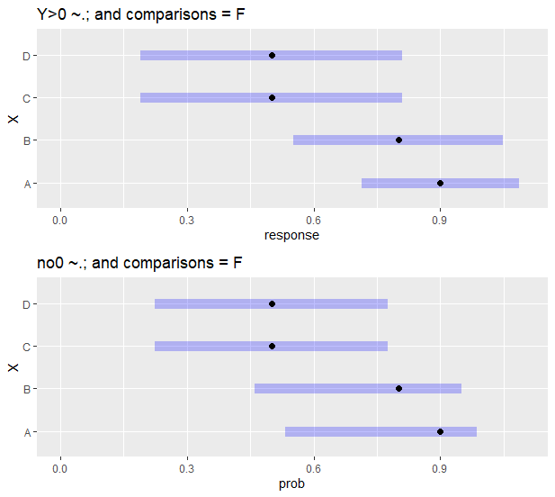
另一个有趣的观察是，当我绘制is表示对象时，没有的，plot()函数中的comparisons = T参数，它用不同的置信区间匹配上面的em3和em4输出：

p1 <- plot(em3, comparisons = F) + scale_x_continuous(limits = c(0,1.1)) + ggtitle("Y>0 ~.; and comparisons = F")
p2 <- plot(em4, comparisons = F) + scale_x_continuous(limits = c(0,1.1)) + ggtitle("no0 ~.; and comparisons = F")
gridExtra::grid.arrange(p1, p2, nrow = 2)

​

​

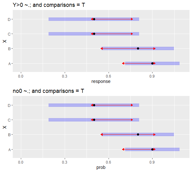
但是当我添加comparisons = T参数时，置信区间现在是相同的，但是两者都匹配基于模型中Y>0规范的模型(参见m3和em3)。

p3 <- plot(em3, comparisons = T) + scale_x_continuous(limits = c(0,1.1)) + ggtitle("Y>0 ~.; and comparisons = T")
p4 <- plot(em4, comparisons = T) + scale_x_continuous(limits = c(0,1.1))+ ggtitle("no0 ~.; and comparisons = T")
gridExtra::grid.arrange(p3, p4, nrow = 2)

​

​

这是有点冗长，但我的问题归结为：

在使用Y>0 ~ X emmeans**，时，可以组合使用模型规范，还是应该首先为此创建一个单独的变量？**

Answer 1

正在发生的情况是， is意味着允许同时存在响应转换和链接函数的情况。例如，当你用伽马族、逆链接和平方根响应变换来拟合一个模型时，这是很方便的。但是，在这种情况下，>被视为响应转换：

> emm1 <- emmeans(m1, "X")

> str(emm1)
'emmGrid' object with variables:
    X = A, B, C, D
Transformation: “logit” 
Additional response transformation: “>” 

当您指定type = "response"时，summary.emmGrid()尝试撤消这两个转换--也就是说，尝试将其放到Y规模上。您可以撤消链接函数，如下所示：

> confint(emm1, type = "unlink")
 X response     SE  df asymp.LCL asymp.UCL
 A      0.9 0.0949 Inf     0.533     0.986
 B      0.8 0.1265 Inf     0.459     0.950
 C      0.5 0.1581 Inf     0.225     0.775
 D      0.5 0.1581 Inf     0.225     0.775

Confidence level used: 0.95 
Intervals are back-transformed from the logit scale 

..。或者通过删除第二个转换：

> emm1a <- update(emm1, tran2 = NULL)
> confint(emm1a, type = "response")
 X response     SE  df asymp.LCL asymp.UCL
 A      0.9 0.0949 Inf     0.533     0.986
 B      0.8 0.1265 Inf     0.459     0.950
 C      0.5 0.1581 Inf     0.225     0.775
 D      0.5 0.1581 Inf     0.225     0.775

Confidence level used: 0.95 
Intervals are back-transformed from the logit scale 

在这两种情况下，这里的置信区间都是在链接标度上计算的，然后再进行反变换.您在这里看到的其他置信限是在以下步骤反转后得到的，即使用反变换结果的标准误差：

> confint(regrid(emm1, transform = "unlink"))
 X response     SE  df asymp.LCL asymp.UCL
 A      0.9 0.0949 Inf     0.714      1.09
 B      0.8 0.1265 Inf     0.552      1.05
 C      0.5 0.1581 Inf     0.190      0.81
 D      0.5 0.1581 Inf     0.190      0.81

Results are given on the > (not the response) scale. 
Confidence level used: 0.95 

我将考虑是否可以进行更改，从而可靠地确定响应转换显然不是有意的。