超高斯拟合

Question

我得研究激光束的轮廓。为了达到这个目的，我需要找到一条适合我的数据的超高斯曲线。超高斯方程：

I * exp(- 2 * ((x - x0) /sigma)^P)

其中P考虑了平顶激光束的曲线特性.

我开始用Python对我的曲线进行简单的高斯拟合。拟合返回高斯曲线，其中对I、x0和sigma的值进行了优化。(我使用函数curve_fit)高斯曲线方程：

I * exp(-(x - x0)^2 / (2 * sigma^2))

现在，我想向前迈出一步。，我想做超高斯曲线拟合，因为我需要考虑光束的平顶特性。因此，我需要一个拟合，它也优化了P参数。

有人知道如何做一个与Python匹配的超高斯曲线吗？

我知道有一种方法可以用做一个超高斯拟合，这不是开源。我没有。因此，我也想知道，如果有人知道一个开源软件，这是可以做一个超高斯曲线拟合或执行。

谢谢

Answer 1

那么，您需要编写一个函数来计算参数化的超高斯，并使用它来建模数据，比如使用scipy.optimize.curve_fit。作为LMFIT (https://lmfit.github.io/lmfit-py/)的主要作者，它为拟合和曲线拟合提供了一个高级接口，我建议您尝试这个库。使用这种方法，您的超级高斯模型函数和用于拟合数据的模型函数可能如下所示：

import numpy as np  
from lmfit import Model   

def super_gaussian(x, amplitude=1.0, center=0.0, sigma=1.0, expon=2.0):
    """super-Gaussian distribution
    super_gaussian(x, amplitude, center, sigma, expon) =
        (amplitude/(sqrt(2*pi)*sigma)) * exp(-abs(x-center)**expon / (2*sigma**expon))
    """
    sigma = max(1.e-15, sigma)
    return ((amplitude/(np.sqrt(2*np.pi)*sigma))
            * np.exp(-abs(x-center)**expon / 2*sigma**expon))

# generate some test data
x = np.linspace(0, 10, 101)
y = super_gaussian(x, amplitude=7.1, center=4.5, sigma=2.5, expon=1.5)
y += np.random.normal(size=len(x), scale=0.015)

# make Model from the super_gaussian function
model = Model(super_gaussian)

# build a set of Parameters to be adjusted in fit, named from the arguments 
# of the model function (super_gaussian), and providing initial values
params = model.make_params(amplitude=1, center=5, sigma=2., expon=2)

# you can place min/max bounds on parameters
params['amplitude'].min = 0
params['sigma'].min = 0
params['expon'].min = 0
params['expon'].max = 100

# note: if you wanted to make this strictly Gaussian, you could set 
# expon=2  and prevent it from varying in the fit:
### params['expon'].value = 2.0
### params['expon'].vary = False

# now do the fit
result = model.fit(y, params, x=x)

# print out the fit statistics, best-fit parameter values and uncertainties
print(result.fit_report())

# plot results
import matplotlib.pyplot as plt
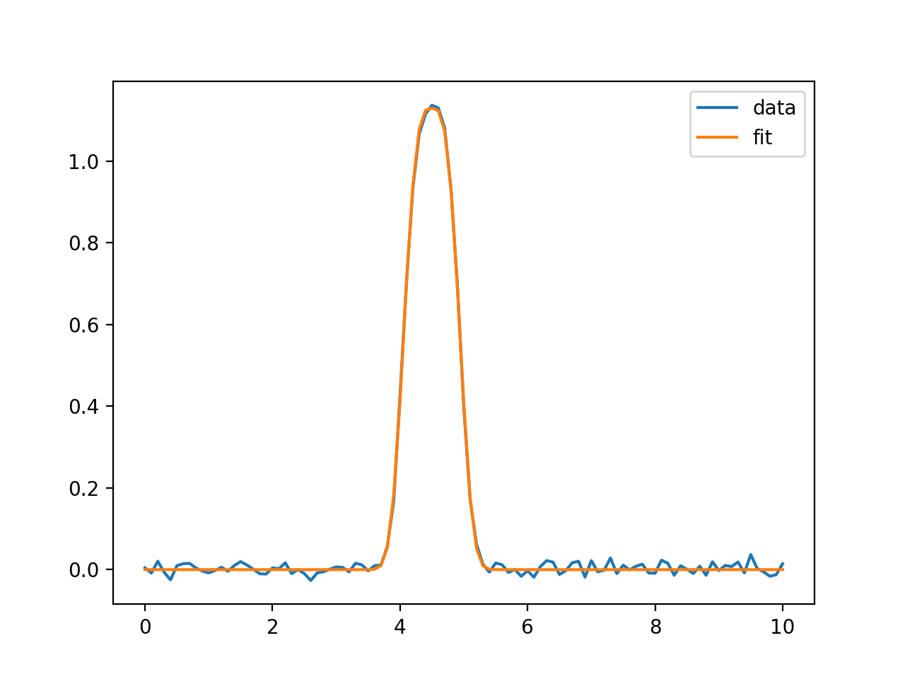
plt.plot(x, y, label='data')
plt.plot(x, result.best_fit, label='fit')
plt.legend()
plt.show()

这将打印一个报告，如

[[Model]]
    Model(super_gaussian)
[[Fit Statistics]]
    # fitting method   = leastsq
    # function evals   = 53
    # data points      = 101
    # variables        = 4
    chi-square         = 0.02110713
    reduced chi-square = 2.1760e-04
    Akaike info crit   = -847.799755
    Bayesian info crit = -837.339273
[[Variables]]
    amplitude:  6.96892162 +/- 0.09939812 (1.43%) (init = 1)
    center:     4.50181661 +/- 0.00217719 (0.05%) (init = 5)
    sigma:      2.48339218 +/- 0.02134446 (0.86%) (init = 2)
    expon:      3.25148164 +/- 0.08379431 (2.58%) (init = 2)
[[Correlations]] (unreported correlations are < 0.100)
    C(amplitude, sigma) =  0.939
    C(sigma, expon)     = -0.774
    C(amplitude, expon) = -0.745

生成这样的情节

​

​

Answer 2

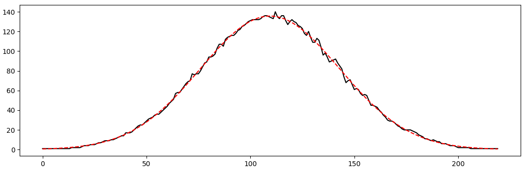
这是超高斯的函数。

    def super_gaussian(x, amp, x0, sigma):
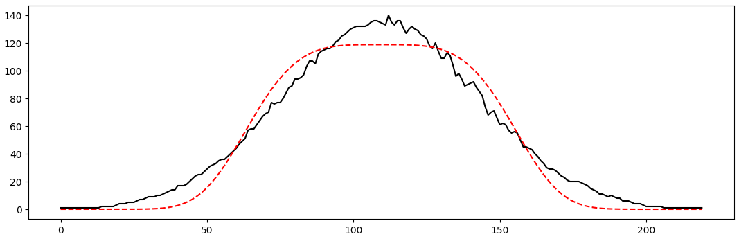
        rank = 2
        return amp * ((np.exp(-(2 ** (2 * rank - 1)) * np.log(2) * (((x - x0) ** 2) / ((sigma) ** 2)) ** (rank))) ** 2)

然后你需要用这样的最优曲线拟合来称呼它：

from scipy import optimize

opt, _ = optimize.curve_fit(super_gaussian, x, y)
vals = super_gaussian(x, *opt)

‘'vals’是你需要绘制的，那是拟合的超高斯函数。

这就是你在rank=1中得到的：

​

rank=2：

​

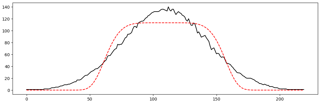
rank=3：

​

Answer 3

纽维尔先生的回答非常适合我。

，但要小心！在super_gaussian函数的定义中，指数的商数中已经出现了抛物。

def super_gaussian(x, amplitude=1.0, center=0.0, sigma=1.0, expon=2.0):
    ...
    return ((amplitude/(np.sqrt(2*np.pi)*sigma))
            * np.exp(-abs(x-center)**expon / 2*sigma**expon))

应代之以

def super_gaussian(x, amplitude=1.0, center=0.0, sigma=1.0, expon=2.0):
    ...
    return (amplitude/(np.sqrt(2*np.pi)*sigma))
           * np.exp(-abs(x-center)**expon / (2*sigma**expon))

然后是超高斯函数的半高宽，它写道：

FWHM = 2.*sigma*(2.*np.log(2.))**(1/expon)

算得很好，与情节非常吻合。

我很抱歉写了这篇课文作为回答。但是我的声誉分数很低，不能给M Newville贴上评论.