计算傅里叶级数来表示数据点

Question

我希望计算一个函数(一个Fourier级数)，它通过一些给定的点集。

类似于这里发生的事情，https://gofigure.impara.ai/，但我不想把它动画化。我只想要这个函数，这样我就可以自己画形状了。我读过很多描述它的数学题和动画的代码，但是我很难实现它。

我的当前代码如下所示，应该能够单独在python笔记本上运行

import matplotlib.pyplot as plt 
import scipy
import cmath 
import math
import numpy as np
from matplotlib import collections  as mc
import pylab as pl


midpoints = [[305.0, 244.5], [293.5, 237.0], [274.5, 367.5], [270.5, 373.5], [229.5, 391.0], [216.0, 396.0], [302.0, 269.0], [295.0, 271.0], [60.5, 146.5], [54.0, 153.0], [52.0, 167.0], [54.0, 153.0], [52.0, 167.0], [45.0, 178.0], [75.0, 76.5], [68.5, 98.5], [75.0, 76.5], [97.0, 58.5], [283.5, 357.5], [274.5, 367.5], [309.0, 255.0], [305.0, 244.5], [309.0, 255.0], [302.0, 269.0], [299.5, 291.5], [300.0, 297.0], [300.0, 297.0], [295.0, 309.5], [62.5, 105.0], [61.0, 118.5], [62.5, 105.0], [68.5, 98.5], [58.0, 139.0], [60.5, 146.5], [241.0, 111.5], [252.0, 124.5], [256.0, 132.5], [252.0, 124.5], [283.0, 356.0], [283.5, 357.5], [300.0, 290.5], [299.5, 291.5], [300.0, 290.5], [296.0, 280.5], [296.0, 280.5], [295.0, 271.0], [158.0, 387.0], [177.0, 396.5], [197.5, 402.0], [192.5, 403.0], [189.5, 400.5], [192.5, 403.0], [197.5, 402.0], [202.5, 401.0], [214.0, 395.5], [216.0, 396.0], [202.5, 401.0], [214.0, 395.5], [233.5, 375.0], [229.5, 391.0], [233.5, 375.0], [249.0, 372.5], [282.5, 340.0], [284.5, 328.0], [284.5, 328.0], [295.0, 309.5], [45.0, 178.0], [49.5, 189.0], [57.0, 198.0], [49.5, 189.0], [238.5, 108.5], [241.0, 111.5], [162.0, 57.5], [170.0, 59.0], [239.5, 204.5], [239.0, 200.0], [293.5, 237.0], [291.0, 227.5], [265.0, 229.5], [291.0, 227.5], [239.0, 189.5], [245.5, 178.0], [239.0, 189.5], [241.0, 193.5], [241.0, 193.5], [239.0, 200.0], [55.0, 119.0], [61.0, 118.5], [53.5, 134.0], [58.0, 139.0], [50.0, 129.0], [55.0, 119.0], [50.0, 129.0], [53.5, 134.0], [107.0, 46.0], [119.5, 50.5], [97.0, 54.0], [97.0, 58.5], [107.0, 46.0], [97.0, 54.0], [150.5, 377.0], [158.0, 387.0], [257.5, 367.5], [270.5, 373.5], [249.0, 372.5], [257.5, 367.5], [280.0, 349.5], [282.5, 340.0], [280.0, 349.5], [283.0, 356.0], [239.5, 90.0], [238.5, 98.0], [238.5, 108.5], [238.5, 98.0], [130.0, 49.0], [119.5, 50.5], [189.0, 65.0], [191.0, 64.5], [189.0, 65.0], [177.0, 62.5], [170.0, 59.0], [177.0, 62.5], [256.0, 132.5], [257.5, 139.5], [128.0, 361.5], [127.5, 360.0], [136.5, 382.5], [131.5, 378.5], [126.5, 370.0], [131.5, 378.5], [128.0, 361.5], [126.5, 370.0], [105.5, 343.5], [101.0, 324.5], [105.5, 343.5], [121.5, 347.5], [126.0, 353.0], [127.5, 360.0], [121.5, 347.5], [126.0, 353.0], [191.0, 64.5], [198.5, 72.0], [237.5, 83.5], [239.5, 90.0], [145.5, 49.0], [138.5, 49.0], [159.0, 57.0], [162.0, 57.5], [145.5, 49.0], [159.0, 57.0], [265.0, 229.5], [254.5, 220.0], [253.0, 216.5], [254.5, 220.0], [253.0, 216.5], [248.0, 208.5], [248.0, 208.5], [239.5, 204.5], [245.0, 173.5], [245.5, 178.0], [250.0, 158.0], [245.0, 173.5], [257.5, 139.5], [250.0, 158.0], [177.0, 396.5], [181.0, 395.5], [181.0, 395.5], [189.5, 400.5], [147.0, 377.0], [150.5, 377.0], [140.5, 381.5], [147.0, 377.0], [140.5, 381.5], [136.5, 382.5], [92.5, 313.5], [101.0, 324.5], [99.5, 290.0], [92.5, 313.5], [98.0, 271.0], [99.5, 290.0], [134.5, 47.5], [130.0, 49.0], [134.5, 47.5], [138.5, 49.0], [73.0, 222.5], [71.0, 214.5], [107.5, 246.0], [110.5, 248.0], [104.0, 266.5], [98.0, 271.0], [69.0, 209.5], [71.0, 214.5], [226.5, 87.0], [237.5, 83.5], [226.5, 87.0], [205.5, 94.5], [205.5, 94.5], [205.5, 77.5], [198.5, 72.0], [205.5, 77.5], [96.5, 244.5], [107.5, 246.0], [109.0, 265.5], [104.0, 266.5], [108.0, 263.5], [110.5, 248.0], [109.0, 265.5], [108.0, 263.5], [65.0, 205.5], [69.0, 209.5], [57.0, 198.0], [56.0, 201.5], [65.0, 205.5], [56.0, 201.5], [90.0, 240.0], [96.5, 244.5], [83.0, 224.0], [73.0, 222.5], [90.5, 231.5], [83.0, 224.0], [90.0, 240.0], [90.5, 231.5]]

x_list = [ p[0] for p in midpoints ]
y_list = [ p[1] for p in midpoints ]
complexmdpts = [ [p[0]+1j*p[1]] for p in midpoints ]

plt.scatter(x_list, y_list, s=50, marker="x", color='y') 

coefs = np.fft.fftshift(scipy.fft.fft(complexmdpts))
n = len(coefs)
print("coeffs[{}]:\n{}".format(n, coefs[:5]))

#todo: sort coeffs?

# function in terms of t to trace out curve
def f(t):
    ftx=0
    fty=0
    for i in range(-int(n/2), int(n/2)+1):
        ftx+=(coefs[i]*cmath.exp(1j*2*math.pi*i*t/n)).real.tolist()[0]
        fty+=(coefs[i]*cmath.exp(1j*2*math.pi*i*t/n)).imag.tolist()[0]
    return [ftx/n, fty/n]
    

lines = [] # store computed lines segments to approximate function

pft = f(0) # compute first point

t_list = np.linspace(0, 2*math.pi, n) # compute list of dts to use when drawing

for t in t_list: 
    cft = f(t)
#     print("f({}): {} \n".format(t, cft))
    lines.append([cft,pft])
    pft = cft

#draw f(t) approximation
lc = mc.LineCollection(lines)
fig, ax = pl.subplots()
ax.add_collection(lc)
ax.autoscale()
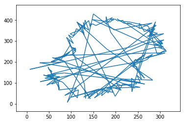
ax.margins(0.1)

这是我的输出：

要点我想概述一下

​

​

My函数逼近

​

​

我不相信快速傅里叶变换是正确使用的。从我所读到的fft是我所需要的，我移动它，因为why返回移位的数组，我认为我的代码的其余部分是正确的，假设系数是正确的，这就是为什么我怀疑这些系数。

在变换和我遗漏的系数之间是否有一步？还是我的函数评估给出的系数不正确？还是我漏掉了什么东西？

Answer 1

实际上，有几个问题需要解决，以获得预期的大纲。让我们逐一讨论一下这些问题。

傅里叶系数计算

由于您正在计算2D数组complexmdpts的FFT (每个元素是一个1复数值的数组)，scipy.fft的默认行为是沿着最后一个轴计算FFT。在这种情况下，这意味着您实际上正在计算长度为1的n FFT，并且如果长度为1的FFT是恒等式，则整个计算将返回原始数组。一种解决方案是显式地指定axis=0：

scipy.fft(complexmdpts,axis=0) 

您也可以将2D数组扁平化为一维数组，因为该数组基本上只有一个维度，但这将导致对基于这个2D结构的代码的其他部分进行更多的更改。

系数移位

当试图解释FFT系数时，有一种常见的混淆。较高指数中的系数对应于出现在奈奎斯特频率之上的环绕后的负频率。为了将这些系数可视化在一个图形上，其中负频率出现在它们直观的位置上，在较高的指数中的系数用fftshift与较低的指数中的系数交换。这样，对应于负频率的系数出现在对应于正频率的系数之前。

在您的具体情况下，f(t)中的计算将负频率(每当i为负，cmath.exp的参数也是负值)与负指数处的系数相关联。由于python数组索引方便地使用从数组末尾计数的元素进行负索引，因此在用负索引进行索引时，您正确地使用了对应于负频率的系数。所有这些都是为了说明不需要用fftshift交换系数，而系数是通过以下方法直接获得的：

coefs = scipy.fft(complexmdpts,axis=0)

采样域

您已经将t指定为从0到2*math.pi。考虑到f(t)的实现，域实际上从0到n (例如，当i==1到cmath.exp的参数从0到1j*2*math.pi时，t从0到n)。要获得跨越整个域的曲线，您应该相应地用以下方法更新t的值：

t_list = np.linspace(0, n, n)

点排序

最后，通过使用散点图绘制原始的一系列点，您隐藏了线条图的外观：

​

​

试图得到一个光滑的函数来插值这个结果，用类似的线条从轮廓的一边跳到另一边。如果你想捕捉这些跳跃，我想你就完了。但我怀疑你很可能想要勾勒出这个地区的轮廓。在这种情况下，您必须对原来的要点进行排序，以便它们遵循大纲。一种方法是迭代地将最近的点附加到先前选定的点。这将给出更接近轮廓的东西：

​

​

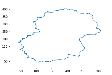
为了演示目的(即不声称这是最好的方法)，您可以使用以下方法进行排序：

def sort_points(points):
  # pick a point
  reference_point = points[0]
  sorted = [reference_point]
  remaining_points = range(1,len(points))
  for i in range(1,len(points)):

    # find the closest point to reference_point, 
    mindiff = np.sum(np.square(np.array(points[remaining_points[0]])-reference_point))
    idx = 0
    # loop over all the other remaining points
    for j in range(1,len(remaining_points)):
      diff = np.sum(np.square(np.array(points[remaining_points[j]])-reference_point))
      if diff < mindiff:
        mindiff = diff
        idx = j        
    # found the closest: update the selected point, and add it to the list of sorted points
    reference_point = points[remaining_points[idx]]
    sorted.append(reference_point )
    remaining_points = np.delete(remaining_points, idx)
  return sorted    

作为参考，以下是完整的代码：

import matplotlib.pyplot as plt 
import scipy
import cmath 
import math
import numpy as np
from matplotlib import collections  as mc
import pylab as pl

def sort_points(points):
  # pick a point
  reference_point = points[0]
  sorted = [reference_point]
  remaining_points = range(1,len(points))
  for i in range(1,len(points)):

    # find the closest point to reference_point, 
    mindiff = np.sum(np.square(np.array(points[remaining_points[0]])-reference_point))
    idx = 0
    # loop over all the other remaining points
    for j in range(1,len(remaining_points)):
      diff = np.sum(np.square(np.array(points[remaining_points[j]])-reference_point))
      if diff < mindiff:
        mindiff = diff
        idx = j        
    # found the closest: update the selected point, and add it to the list of sorted points
    reference_point = points[remaining_points[idx]]
    sorted.append(reference_point )
    remaining_points = np.delete(remaining_points, idx)
  return sorted    


midpoints = [[305.0, 244.5], [293.5, 237.0], [274.5, 367.5], [270.5, 373.5], [229.5, 391.0], [216.0, 396.0], [302.0, 269.0], [295.0, 271.0], [60.5, 146.5], [54.0, 153.0], [52.0, 167.0], [54.0, 153.0], [52.0, 167.0], [45.0, 178.0], [75.0, 76.5], [68.5, 98.5], [75.0, 76.5], [97.0, 58.5], [283.5, 357.5], [274.5, 367.5], [309.0, 255.0], [305.0, 244.5], [309.0, 255.0], [302.0, 269.0], [299.5, 291.5], [300.0, 297.0], [300.0, 297.0], [295.0, 309.5], [62.5, 105.0], [61.0, 118.5], [62.5, 105.0], [68.5, 98.5], [58.0, 139.0], [60.5, 146.5], [241.0, 111.5], [252.0, 124.5], [256.0, 132.5], [252.0, 124.5], [283.0, 356.0], [283.5, 357.5], [300.0, 290.5], [299.5, 291.5], [300.0, 290.5], [296.0, 280.5], [296.0, 280.5], [295.0, 271.0], [158.0, 387.0], [177.0, 396.5], [197.5, 402.0], [192.5, 403.0], [189.5, 400.5], [192.5, 403.0], [197.5, 402.0], [202.5, 401.0], [214.0, 395.5], [216.0, 396.0], [202.5, 401.0], [214.0, 395.5], [233.5, 375.0], [229.5, 391.0], [233.5, 375.0], [249.0, 372.5], [282.5, 340.0], [284.5, 328.0], [284.5, 328.0], [295.0, 309.5], [45.0, 178.0], [49.5, 189.0], [57.0, 198.0], [49.5, 189.0], [238.5, 108.5], [241.0, 111.5], [162.0, 57.5], [170.0, 59.0], [239.5, 204.5], [239.0, 200.0], [293.5, 237.0], [291.0, 227.5], [265.0, 229.5], [291.0, 227.5], [239.0, 189.5], [245.5, 178.0], [239.0, 189.5], [241.0, 193.5], [241.0, 193.5], [239.0, 200.0], [55.0, 119.0], [61.0, 118.5], [53.5, 134.0], [58.0, 139.0], [50.0, 129.0], [55.0, 119.0], [50.0, 129.0], [53.5, 134.0], [107.0, 46.0], [119.5, 50.5], [97.0, 54.0], [97.0, 58.5], [107.0, 46.0], [97.0, 54.0], [150.5, 377.0], [158.0, 387.0], [257.5, 367.5], [270.5, 373.5], [249.0, 372.5], [257.5, 367.5], [280.0, 349.5], [282.5, 340.0], [280.0, 349.5], [283.0, 356.0], [239.5, 90.0], [238.5, 98.0], [238.5, 108.5], [238.5, 98.0], [130.0, 49.0], [119.5, 50.5], [189.0, 65.0], [191.0, 64.5], [189.0, 65.0], [177.0, 62.5], [170.0, 59.0], [177.0, 62.5], [256.0, 132.5], [257.5, 139.5], [128.0, 361.5], [127.5, 360.0], [136.5, 382.5], [131.5, 378.5], [126.5, 370.0], [131.5, 378.5], [128.0, 361.5], [126.5, 370.0], [105.5, 343.5], [101.0, 324.5], [105.5, 343.5], [121.5, 347.5], [126.0, 353.0], [127.5, 360.0], [121.5, 347.5], [126.0, 353.0], [191.0, 64.5], [198.5, 72.0], [237.5, 83.5], [239.5, 90.0], [145.5, 49.0], [138.5, 49.0], [159.0, 57.0], [162.0, 57.5], [145.5, 49.0], [159.0, 57.0], [265.0, 229.5], [254.5, 220.0], [253.0, 216.5], [254.5, 220.0], [253.0, 216.5], [248.0, 208.5], [248.0, 208.5], [239.5, 204.5], [245.0, 173.5], [245.5, 178.0], [250.0, 158.0], [245.0, 173.5], [257.5, 139.5], [250.0, 158.0], [177.0, 396.5], [181.0, 395.5], [181.0, 395.5], [189.5, 400.5], [147.0, 377.0], [150.5, 377.0], [140.5, 381.5], [147.0, 377.0], [140.5, 381.5], [136.5, 382.5], [92.5, 313.5], [101.0, 324.5], [99.5, 290.0], [92.5, 313.5], [98.0, 271.0], [99.5, 290.0], [134.5, 47.5], [130.0, 49.0], [134.5, 47.5], [138.5, 49.0], [73.0, 222.5], [71.0, 214.5], [107.5, 246.0], [110.5, 248.0], [104.0, 266.5], [98.0, 271.0], [69.0, 209.5], [71.0, 214.5], [226.5, 87.0], [237.5, 83.5], [226.5, 87.0], [205.5, 94.5], [205.5, 94.5], [205.5, 77.5], [198.5, 72.0], [205.5, 77.5], [96.5, 244.5], [107.5, 246.0], [109.0, 265.5], [104.0, 266.5], [108.0, 263.5], [110.5, 248.0], [109.0, 265.5], [108.0, 263.5], [65.0, 205.5], [69.0, 209.5], [57.0, 198.0], [56.0, 201.5], [65.0, 205.5], [56.0, 201.5], [90.0, 240.0], [96.5, 244.5], [83.0, 224.0], [73.0, 222.5], [90.5, 231.5], [83.0, 224.0], [90.0, 240.0], [90.5, 231.5]]
midpoints = sort_points(midpoints)

x_list = [ p[0] for p in midpoints ]
y_list = [ p[1] for p in midpoints ]
complexmdpts = [ [p[0]+1j*p[1]] for p in midpoints ]

plt.scatter(x_list, y_list, s=50, marker="x", color='y') 

coefs = scipy.fft(complexmdpts,axis=0)
n = len(coefs)
print("coeffs[{}]:\n{}".format(n, coefs[:5]))

# function in terms of t to trace out curve
m = n
def f(t):
    ftx=0
    fty=0
    for i in range(-int(m/2), int(m/2)+1):
        ftx+=(coefs[i]*cmath.exp(1j*2*math.pi*i*t/n)).real.tolist()[0]
        fty+=(coefs[i]*cmath.exp(1j*2*math.pi*i*t/n)).imag.tolist()[0]
    return [ftx/n, fty/n]
    

lines = [] # store computed lines segments to approximate function

pft = f(0) # compute first point

t_list = np.linspace(0, n, n) # compute list of dts to use when drawing

for t in t_list: 
    cft = f(t)
    lines.append([cft,pft])
    pft = cft

#draw f(t) approximation
lc = mc.LineCollection(lines)
fig, ax = pl.subplots()
ax.add_collection(lc)
ax.autoscale()
ax.margins(0.1)