用Rcpp & Kronecker乘积快速计算nnet的Hessian / Fisher信息矩阵:R中的多项式多项式回归

Question

对于较大的nnet::multinom多项式回归模型(具有几千个系数)，计算Hessian (负对数似然的二阶导数矩阵，也称为观测的费雪信息矩阵)变得超慢，从而使我无法计算方差协方差矩阵，从而使我能够计算模型预测的置信区间。

罪魁祸首似乎是以下纯R函数--它似乎使用一些代码来解析地计算费舍尔信息矩阵，使用David：https://github.com/cran/nnet/blob/master/R/vcovmultinom.R提供的代码

multinomHess = function (object, Z = model.matrix(object)) 
{
    probs <- object$fitted
    coefs <- coef(object)
    if (is.vector(coefs)) {
        coefs <- t(as.matrix(coefs))
        probs <- cbind(1 - probs, probs)
    }
    coefdim <- dim(coefs)
    p <- coefdim[2L]
    k <- coefdim[1L]
    ncoefs <- k * p
    kpees <- rep(p, k)
    n <- dim(Z)[1L]

##  Now compute the observed (= expected, in this case) information,
##  e.g. as in T Amemiya "Advanced Econometrics" (1985) pp 295-6.
##  Here i and j are as in Amemiya, and x, xbar are vectors
##  specific to (i,j) and to i respectively.

    info <- matrix(0, ncoefs, ncoefs)
    Names <- dimnames(coefs)
    if (is.null(Names[[1L]])) 
        Names <- Names[[2L]]
    else Names <- as.vector(outer(Names[[2L]], Names[[1L]], function(name2, 
        name1) paste(name1, name2, sep = ":")))
    dimnames(info) <- list(Names, Names)
    x0 <- matrix(0, p, k + 1L)
    row.totals <- object$weights
    for (i in seq_len(n)) {
        Zi <- Z[i, ]
        xbar <- rep(Zi, times=k) * rep(probs[i, -1, drop=FALSE], times=kpees)
        for (j in seq_len(k + 1)) {
            x <- x0
            x[, j] <- Zi
            x <- x[, -1, drop = FALSE]
            x <- x - xbar
            dim(x) <- c(1, ncoefs)
            info <- info + (row.totals[i] * probs[i, j] * crossprod(x))
        }
    }
    info
}

参考状态的高级计量经济学书籍中的信息

​

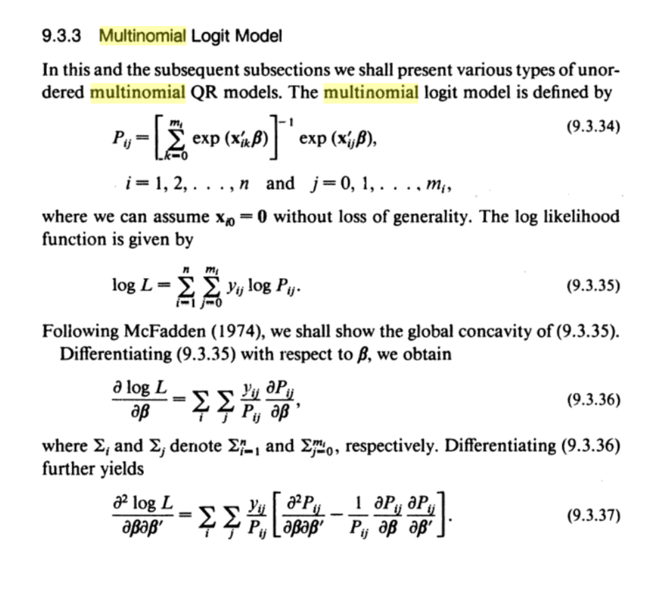
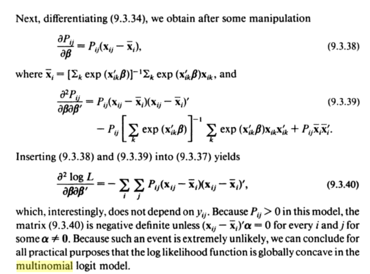
从这个解释中，我们可以看到，Hessian确实是由一群交叉乘积之和给出的。在如何计算多项式回归模型的Hessian矩阵方面，我还看到了这和这，这可能更加优雅和有效，因为Hessian是根据Kronecker积之和计算的。

对于一个小型的nnet::multinom模型(在这个模型中，我正在模拟不同SARS 2谱系的频率随时间变化)，所提供的函数运行得很快：

library(nnet)
library(splines)
download.file("https://www.dropbox.com/s/gt0yennn2gkg3rd/smallmodel.RData?dl=1",
              "smallmodel.RData", 
              method = "auto", mode="wb")
load("smallmodel.RData")
length(fit_multinom_small$lev) # k=12 outcome levels
dim(coef(fit_multinom_small)) # 11 x 3 = (k-1) x p = 33 coefs
system.time(hess <- nnet:::multinomHess(fit_multinom_small)) # 0.11s
dim(hess) # 33 33

但是，对一个大型模型这样做需要超过2个小时(即使模型本身适合于大约1分钟)(再次模拟不同的SARS-CoV2 2谱系在时间上的频率，但现在跨越不同的大陆/国家)：

download.file("https://www.dropbox.com/s/mpz08jj7fmubd68/bigmodel.RData?dl=1",
              "bigmodel.RData", 
              method = "auto", mode="wb")
load("bigmodel.RData")
length(fit_global_multi_last3m$lev) # k=20 outcome levels
dim(coef(fit_global_multi_last3m)) # 19 x 229 = (k-1) x p = 4351 coefficients
system.time(hess <- nnet:::multinomHess(fit_global_multi_last3m)) # takes forever

我现在正在寻找加速上述功能的方法。

显而易见的尝试可能是将其移植到Rcpp，但不幸的是，我在这方面没有这么多经验。有人有什么想法吗？

编辑:从info 这里和这里上看，计算多项式拟合的Hessian值应该可以归结为计算Kronecker乘积的和，我们可以用有效的矩阵代数从R开始计算，但是现在我还不确定如何包含总行数fit$weights。有人知道吗？

download.file("https://www.dropbox.com/s/gt0yennn2gkg3rd/smallmodel.RData?dl=1",
                      "smallmodel.RData", 
                      method = "auto", mode="wb")

load("smallmodel.RData")
library(nnet)
length(fit_multinom_small$lev) # k=12 outcome levels
dim(coef(fit_multinom_small)) # 11 x 3 = (k-1) x p = 33 coefs

fit = fit_multinom_small

Z = model.matrix(fit)
P = fitted(fit)[, -1, drop=F]
k = ncol(P) # nr of outcome categories-1
p = ncol(Z) # nr of parameters
n = nrow(Z) # nr of observations
ncoefs = k*p
library(fastmatrix)

# Fisher information matrix
info <- matrix(0, ncoefs, ncoefs)
for (i in 1:n) { # sum over observations
info = info + kronecker.prod(diag(P[i,]) - tcrossprod(P[i,]), tcrossprod(Z[i,]))
}

Answer 1

最终发现了&能够使用Kronecker产品计算观察到的Fisher信息矩阵，以及使用Armadillo类计算到Rcpp的端口(完全公开:我只使用OpenAI代码-davinci/ Codex、https://openai.com/blog/openai-codex/，令人惊讶的是，它的效果越来越好-- AI每天都在变得更好；parallelReduce仍然可以用来并行我假设的积累；函数比我尝试过的类似的RcppEigen实现更快)。我犯的错误是，上面的公式是观测到的一个观测的Fisher信息，所以我必须在观察的基础上进行积累&我还必须考虑到我的总行数。

Rcpp功能：

// RcppArmadillo utility function to calculate observed Fisher 
// information matrix of multinomial fit, with 
// probs=fitted probabilities (with 1st category/column dropped)
// Z = model matrix
// row_totals = row totals
// We do this using Kronecker products, as in
// https://ieeexplore.ieee.org/abstract/document/1424458
// B. Krishnapuram; L. Carin; M.A.T. Figueiredo; A.J. Hartemink
// Sparse multinomial logistic regression: fast algorithms and
// generalization bounds
// IEEE Transactions on Pattern Analysis and Machine
// Intelligence ( Volume: 27, Issue: 6, June 2005)

#include <RcppArmadillo.h>

using namespace arma;

// [[Rcpp::depends(RcppArmadillo)]]
// [[Rcpp::export]]
arma::mat calc_infmatrix_RcppArma(arma::mat probs, arma::mat Z, arma::vec row_totals) {
  int n = Z.n_rows;
  int p = Z.n_cols;
  int k = probs.n_cols;
  int ncoefs = k * p;
  arma::mat info = arma::zeros<arma::mat>(ncoefs, ncoefs);
  arma::mat diag_probs;
  arma::mat tcrossprod_probs;
  arma::mat tcrossprod_Z;
  arma::mat kronecker_prod;
  for (int i = 0; i < n; i++) {
    diag_probs = arma::diagmat(probs.row(i));
    tcrossprod_probs = arma::trans(probs.row(i)) * probs.row(i);
    tcrossprod_Z = (arma::trans(Z.row(i)) * Z.row(i)) * row_totals(i);
    kronecker_prod = arma::kron(diag_probs - tcrossprod_probs, tcrossprod_Z);
    info += kronecker_prod;
  }
  return info;
}

保存为"calc_infmatrix_arma.cpp"。

library(Rcpp)
library(RcppArmadillo)
sourceCpp("calc_infmatrix_arma.cpp")

R包装函数：

# Function to calculate Hessian / observed Fisher information
# matrix of nnet::multinom multinomial fit object
fastmultinomHess <- function(object, Z = model.matrix(object)) {
  
  probs <- object$fitted # predicted probabilities, avoid napredict from fitted.default

  coefs <- coef(object)
  if (is.vector(coefs)){ # ie there are only 2 response categories
    coefs <- t(as.matrix(coefs))
    probs <- cbind(1 - probs, probs)
  }
  coefdim <- dim(coefs)
  p <- coefdim[2L] # nr of parameters
  k <- coefdim[1L] # nr out outcome categories-1
  ncoefs <- k * p # nr of coefficients
  n <- dim(Z)[1L] # nr of observations
  
  #  Now compute the Hessian = the observed 
  #  (= expected, in this case) 
  #  Fisher information matrix
    
  info <- calc_infmatrix_RcppArma(probs = probs[, -1, drop=F], 
                                  Z = Z, 
                                  row_totals = object$weights)

  Names <- dimnames(coefs)
  if (is.null(Names[[1L]])) Names <- Names[[2L]] else Names <- as.vector(outer(Names[[2L]], Names[[1L]],
                                function(name2, name1)
                                  paste(name1, name2, sep = ":")))
  dimnames(info) <- list(Names, Names)

  return(info)
}

对于我的更大的模型，它现在计算在100，而不是>2小时，所以几乎快了80倍：

download.file("https://www.dropbox.com/s/mpz08jj7fmubd68/bigmodel.RData?dl=1",
              "bigmodel.RData", 
              method = "auto", mode="wb")
load("bigmodel.RData")
object = fit_global_multi_last3m # large nnet::multinom fit
system.time(info <- fastmultinomHess(object, Z = model.matrix(object))) # 103s
system.time(info <- nnet:::multinomHess(object, Z = model.matrix(object))) # 8127s = 2.25h

calc_infmatrix函数的纯R版本(比上面的Rcpp函数慢约5x )将是

# Utility function to calculate observed Fisher information matrix
# of multinomial fit, with 
# probs=fitted probabilities (with 1st category/column dropped)
# Z = model matrix
# row_totals = row totals
    calc_infmatrix = function(probs, Z, row_totals) {
      require(fastmatrix) # for kronecker.prod Kronecker product function
      
      n <- nrow(Z)
      p <- ncol(Z)
      k <- ncol(probs)
      ncoefs <- k * p
      info <- matrix(0, ncoefs, ncoefs)
      for (i in 1:n) {
        info <- info + kronecker.prod((diag(probs[i,]) - tcrossprod(probs[i,])), tcrossprod(Z[i,])*row_totals[i] )
      }
      return(info)  
    }