三元空间中的Plotly回归

Question

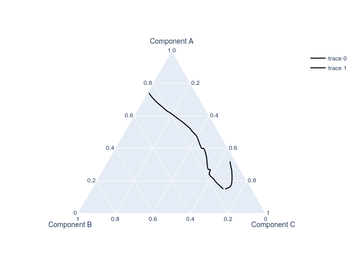
我试图在三元空间中用python巧妙地绘制一条回归线，但对于散乱三元，似乎没有“趋势线=‘黄土’”这样的选项。是否有另一种方法可以实现三元流的同样结果呢?前一篇文章中的代码生成了样条线，而不是回归线。

import numpy as np
import plotly.graph_objects as go

a = np.array([0.15, 0.15, 0.17, 0.2 , 0.21, 0.24, 0.26, 0.27, 0.27, 0.29, 0.32, 0.35, 0.39, 0.4 , 0.4 , 0.41, 0.47, 0.48, 0.51, 0.52, 0.54, 0.56, 0.59, 0.62, 0.63, 0.65, 0.69, 0.73, 0.74])
b = np.array([0.14, 0.15, 0.1 , 0.17, 0.17, 0.18, 0.05, 0.16, 0.17, 0.04, 0.03, 0.14, 0.13, 0.13, 0.14, 0.14, 0.13, 0.13, 0.14, 0.14, 0.15, 0.16, 0.18, 0.2 , 0.21, 0.22, 0.24, 0.25, 0.25])
c = np.array([0.71, 0.7 , 0.73, 0.63, 0.62, 0.58, 0.69, 0.57, 0.56, 0.67, 0.65, 0.51, 0.48, 0.47, 0.46, 0.45, 0.4 , 0.39, 0.35, 0.34, 0.31, 0.28, 0.23, 0.18, 0.16, 0.13, 0.07, 0.02, 0.01])

fig = go.Figure()

curve_portion = np.where((b < 0.15) & (c > 0.6))
curve_other_portion = np.where(~((b < 0.15) & (c > 0.6)))

def add_plot_spline_portions(fig, indices_groupings):
    for indices in indices_groupings:
        fig.add_trace(go.Scatterternary({
            'mode': 'lines',
            'connectgaps': True,
            'a': a[indices],
            'b': b[indices],
            'c': c[indices],
            'line': {'color': 'black', 'shape': 'spline', 'smoothing': 1},
            'marker': {'size': 2, 'line': {'width': 0.1}}
            })
            )    

add_plot_spline_portions(fig, [curve_portion, curve_other_portion])
fig.show(renderer='png')

​

​

Answer 1

我可以勾勒出我认为是一种一般的解决方案--它没有我想要的那么严格的数学，并且涉及一些猜测和检查类型的工作--但希望它是有帮助的。

首先要考虑的是，对于三元图上的这种回归，只有两个自由度，因为A+B+C=1 (您可能会发现这一解释很有用)。这意味着一次只考虑两个变量之间的关系是有意义的。我们真正想要做的是在两个变量之间建立一个回归，然后使用方程A+B+C=1确定第三个变量的值。

第二个考虑因素是很难定义的，但是由于您是在一个包含变量A的“反转”性质的回归之后，所以我们需要一个回归，其中A可以接受重复的值。我认为实现这一目标的最直接的方法是A是你所预测的变量。

为了简单起见，假设我们使用了一个从B或C中预测A的2次多项式回归，我们可以进行散射，并选择哪个多项式更适合我们的目的。

下面是一篇简短的文章：

import numpy as np
import plotly.graph_objects as go
from plotly.subplots import make_subplots

a = np.array([0.15, 0.15, 0.17, 0.2 , 0.21, 0.24, 0.26, 0.27, 0.27, 0.29, 0.32, 0.35, 0.39, 0.4 , 0.4 , 0.41, 0.47, 0.48, 0.51, 0.52, 0.54, 0.56, 0.59, 0.62, 0.63, 0.65, 0.69, 0.73, 0.74])
b = np.array([0.14, 0.15, 0.1 , 0.17, 0.17, 0.18, 0.05, 0.16, 0.17, 0.04, 0.03, 0.14, 0.13, 0.13, 0.14, 0.14, 0.13, 0.13, 0.14, 0.14, 0.15, 0.16, 0.18, 0.2 , 0.21, 0.22, 0.24, 0.25, 0.25])
c = np.array([0.71, 0.7 , 0.73, 0.63, 0.62, 0.58, 0.69, 0.57, 0.56, 0.67, 0.65, 0.51, 0.48, 0.47, 0.46, 0.45, 0.4 , 0.39, 0.35, 0.34, 0.31, 0.28, 0.23, 0.18, 0.16, 0.13, 0.07, 0.02, 0.01])

## eda to determine polynomial of best fit to predict A 
fig_eda = make_subplots(rows=1, cols=2)

fig_eda.add_trace(go.Scatter(x=b, y=a, mode='markers'),row=1, col=1)
coefficients = np.polyfit(b,a,2)
p = np.poly1d(coefficients)
b_vals = np.linspace(min(b),max(b))
a_pred = np.array([p(x) for x in b_vals])
fig_eda.add_trace(go.Scatter(x=b_vals, y=a_pred, mode='lines'),row=1, col=1)

fig_eda.add_trace(go.Scatter(x=c, y=a, mode='markers'),row=1, col=2)
coefficients = np.polyfit(c,a,2)
p = np.poly1d(coefficients)
c_vals = np.linspace(min(c),max(c))
a_pred = np.array([p(x) for x in c_vals])
fig_eda.add_trace(go.Scatter(x=c_vals, y=a_pred, mode='lines'),row=1, col=2)

​

​

注意，predicting A from B看起来比从C中预测A更好地捕捉了A的反转性质，如果我们尝试对C的A进行2次多项式回归，我们可以看到A不会在C: 0,1的范围内重复，因为该多项式的斜率很低。

让我们继续这个回归，C作为预测变量，A作为预测变量(B也是使用B = 1 - (A + C)的预测变量。

fig = go.Figure()

fig.add_trace(go.Scatterternary({
    'mode': 'markers',
    'connectgaps': True,
    'a': a,
    'b': b,
    'c': c
}))   

## since A+B+C = 100, we only need to fit a polynomial between two of the variables
## fit an n-degree polynomial to 2 of your variables
## source https://numpy.org/doc/stable/reference/generated/numpy.polyfit.html

coefficients = np.polyfit(b,a,2)
p = np.poly1d(coefficients)

## we use the entire domain of the input variable B
b_vals = np.linspace(0,1)

a_pred = np.array([p(x) for x in b_vals])
c_pred = 1 - (b_vals + a_pred)

fig.add_trace(go.Scatterternary({
    'mode': 'lines',
    'connectgaps': True,
    'a': a_pred,
    'b': b_vals,
    'c': c_pred,
    'marker': {'size': 2, 'color':'red', 'line': {'width': 0.1}}
}))   

fig.show()

​

​

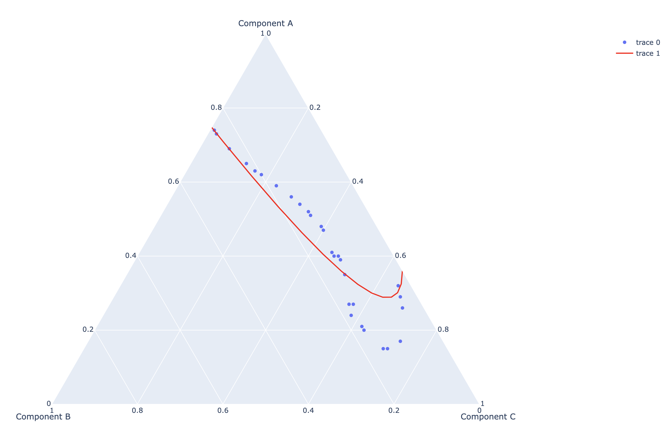
这是允许A的重复值的最低次多项式回归(预测A的线性回归就是不允许A接受重复值)。然而，你绝对可以尝试增加你所使用的多项式的程度，并从变量B或C中预测A。