气候指数计算教程:SPI、SPEI 与 PET 的实现

气候指数计算教程:SPI、SPEI 与 PET 的实现

用户11172986
发布于 2026-04-24 19:21:30
发布于 2026-04-24 19:21:30
气候指数计算教程:SPI、SPEI 与 PET 的实现
温馨提示
- 由于可视化代码过长隐藏,可点击运行Fork查看
- 若没有成功加载可视化图,点击运行可以查看
- ps:隐藏代码在【代码已被隐藏】所在行,点击所在行,可以看到该行的最右角,会出现个三角形,点击查看即可
项目背景:
本项目旨在解决气候研究中降水、气象干旱及蒸散发等指数的计算问题。通过 Python 的 climate-indices 库,我们可以高效地处理网格化气象数据。
1. 环境准备
首先,安装必要的库。由于 climate-indices 对版本有特定要求,建议在独立的环境中运行。
!pip install climate-indices -i https://pypi.mirrors.ustc.edu.cn/simple/
这个项目包含了多种气候指数算法的 Python 实现,这些算法提供了降水和温度异常严重程度的地理和时间分布图,适用于气候监测和研究。
提供的指数包括:
- SPI(标准化降水指数):利用伽玛分布和皮尔逊 III 型分布。
- SPEI(标准化降水蒸散指数):利用伽玛分布和皮尔逊 III 型分布。
- PET(潜在蒸发散):利用 Thornthwaite 方程或 Hargreaves 方程。
- PNP(正常降水百分比)。
2. 拟造模拟数据
为了演示计算过程,我们使用 xarray 构建一个包含 30 年月尺度降水和气温的模拟数据集。
import numpy as np
import pandas as pd
import xarray as xr

# 1. 设定时间范围(30年,月频率)
times = pd.date_range("1991-01-01", "2020-12-31", freq="MS")
lats = np.array([30.0, 31.0])
lons = np.array([110.0, 111.0])

# --- 修复部分 ---
# 将 times.month 转换为 numpy 数组,再进行维度扩展 [:, None, None]
# 这样是为了将 (360,) 形状的数组变成 (360, 1, 1),以便与 (360, 2, 2) 的格点数据对齐
month_values = times.month.values  # 转换为 numpy 数组
seasonal_cycle = np.sin(2 * np.pi * month_values / 12)
seasonal_cycle_3d = seasonal_cycle[:, None, None]
# ----------------

# 2. 模拟降水数据 (单位: mm) - 包含季节性
np.random.seed(42)
# 降水通常也有季节性,这里简单模拟
precip_base = 50 + 40 * seasonal_cycle_3d
precip_data = np.maximum(0, precip_base + np.random.normal(0, 15, (len(times), len(lats), len(lons))))

# 3. 模拟气温数据 (单位: Celsius) - 修复后的写法
temp_data = 15 + 10 * seasonal_cycle_3d + np.random.normal(0, 2, (len(times), len(lats), len(lons)))

# 4. 封装进 xarray Dataset
ds = xr.Dataset(
    {
        "precip": (["time", "lat", "lon"], precip_data),
        "temp": (["time", "lat", "lon"], temp_data),
    },
    coords={
        "time": times,
        "lat": lats,
        "lon": lons,
    },
)

print("数据集成功创建!")
print(ds)
3. 计算潜在蒸散发 (PET)
PET 是计算 SPEI 的基础。我们使用 Thornthwaite 算法,该算法仅需要气温和纬度。
from climate_indices import indices
from climate_indices import compute
# 提取其中一个格点的数据
selected_lat = ds.lat.values[0]
temp_series = ds.temp.sel(lat=selected_lat, lon=110.0).values

# 在 climate-indices 2.0.0 中,计算 PET 的方式如下:
# 我们需要指定 pet_type (如 thornthwaite)
pet = indices.pet(
    temperature_celsius=temp_series,
    latitude_degrees=selected_lat,
    data_start_year=1991# 对应我们模拟数据的开始年份
)

print(f"PET 计算成功!前5个月数值: {pet[:5]}")
4. 计算标准化降水指数 (SPI)
SPI 衡量降水偏离正常水平的程度。
precip_series = ds.precip.sel(lat=30.0, lon=110.0).values

# 计算 3 个月尺度的 SPI
spi_3 = indices.spi(
    values=precip_series,
    scale=3,
    distribution=indices.Distribution.gamma,
    data_start_year=1991,
    calibration_year_initial=1991,
    calibration_year_final=2020,
    periodicity=compute.Periodicity.monthly  # <--- 新增这个参数
)

print(f"SPI-3 计算成功!前5个月数值:\n{spi_3[:5]}")
5. 计算标准化降水蒸散指数 (SPEI)
SPEI 结合了降水和 PET 的差值(D = P - PET),能更好地反映气温升高对干旱的影响。
spei_6 = indices.spei(precips_mm=precip_series,
                    pet_mm=pet,
                    scale=6, # 6个月尺度
                    distribution=indices.Distribution.gamma,
                    periodicity=compute.Periodicity.monthly,
                    data_start_year=1991,
                    calibration_year_initial=1991,
                    calibration_year_final=2020,
                    )
print(f"前10个月的 SPEI-6 结果: {spei_3[:10]}")
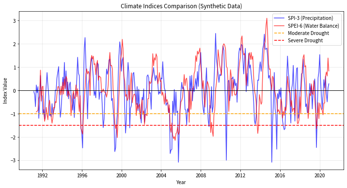
6. 结果可视化
将计算出的 SPI 和 SPEI 进行对比绘图。
import matplotlib.pyplot as plt

plt.figure(figsize=(12, 6))

# 设置绘图时间轴
plot_times = ds.time.values

plt.plot(plot_times, spi_3, label='SPI-3 (Precipitation)', alpha=0.7, color='blue')
plt.plot(plot_times, spei_6, label='SPEI-6 (Water Balance)', alpha=0.7, color='red')

# 添加 0 基准线和旱涝阈值
plt.axhline(0, color='black', linestyle='-', linewidth=1)
plt.axhline(-1, color='orange', linestyle='--', label='Moderate Drought')
plt.axhline(-1.5, color='red', linestyle='--', label='Severe Drought')

plt.title("Climate Indices Comparison (Synthetic Data)")
plt.xlabel("Year")
plt.ylabel("Index Value")
plt.legend()
plt.grid(True, alpha=0.3)
plt.show()
No description has been provided for this image
7. 注意事项
- 数据长度:计算 SPI/SPEI 时,建议至少使用 30 年以上的数据作为校准期。
- 缺失值:climate-indices 在处理缺失值时比较敏感,请确保输入数据已进行预处理。
- 库版本依赖:如安装日志所示,该库对 numpy, scipy 和 xarray 的版本有严格要求,由于这些版本较旧,建议在独立的 Docker 容器或 conda 环境中进行实验,避免影响其他项目。
本文参与 腾讯云自媒体同步曝光计划,分享自微信公众号。
原始发表:2026-01-10,如有侵权请联系 cloudcommunity@tencent.com 删除
评论
登录后参与评论
推荐阅读
目录
腾讯云开发者

Copyright © 2013 - 2026 Tencent Cloud. All Rights Reserved. 腾讯云 版权所有
深圳市腾讯计算机系统有限公司 ICP备案/许可证号:粤B2-20090059 ![]() 粤公网安备44030502008569号
粤公网安备44030502008569号
腾讯云计算(北京)有限责任公司 京ICP证150476号 | 京ICP备11018762号