苹果进军蛋白质折叠:SimpleFold 使用体验

苹果进军蛋白质折叠:SimpleFold 使用体验

Tom2Code
发布于 2026-04-17 17:31:50
发布于 2026-04-17 17:31:50
今天,我们把「简单」带进蛋白质结构预测。
哈哈哈,先模仿一下Apple的语气。今天我们先来读一下论文,然后再部署一下simpleFold玩一下。
一.背景介绍
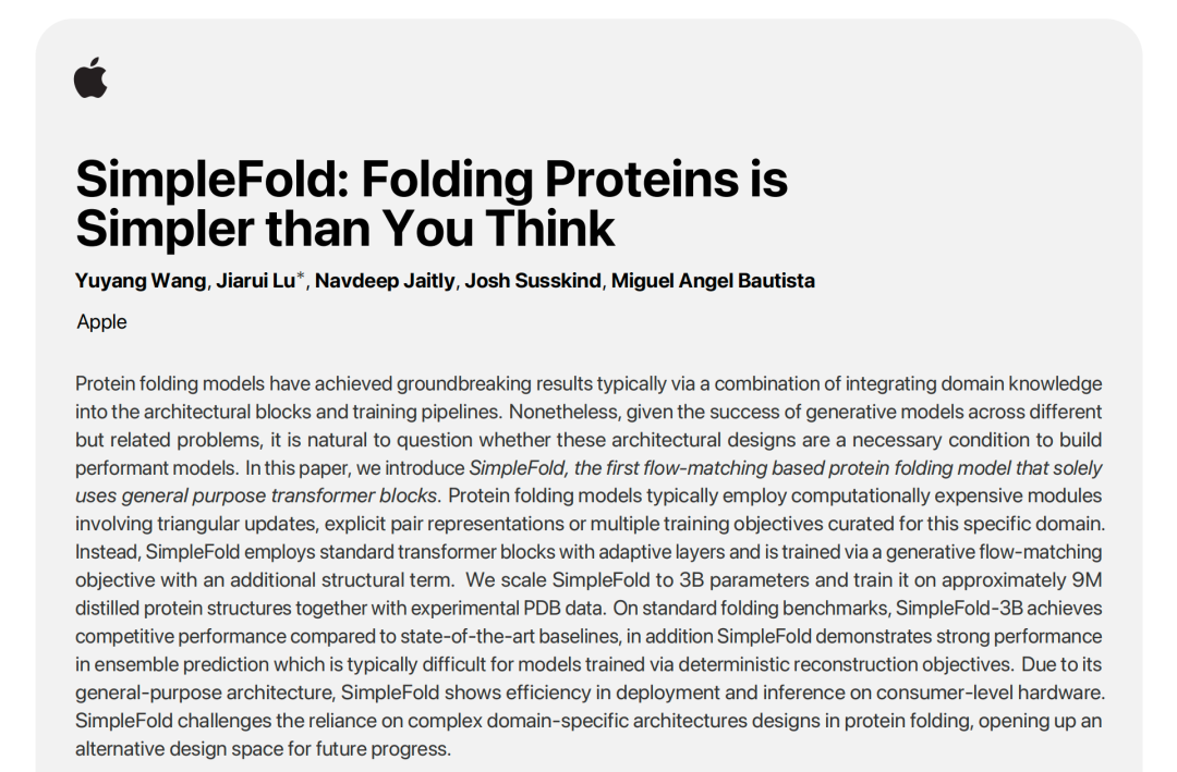
蛋白质折叠是计算生物学中一项长期存在的挑战,对药物研发具有深远影响。过去,高性能的蛋白质折叠模型(如AlphaFold2)通常依赖于集成领域知识和计算成本高昂的架构模块,例如三角更新和显式配对表示。然而,来自 Apple 的研究人员最近推出了 SimpleFold 模型,它挑战了这种对复杂架构的依赖性。SimpleFold 是第一个纯粹基于通用 Transformer 模块和流匹配(flow-matching)目标训练的蛋白质折叠模型。它成功地摒弃了多序列比对(MSA)、配对表示或三角更新等昂贵的特定领域设计,大大降低了架构复杂性。通过扩展到 30 亿参数并在大约 900 万个蒸馏结构上进行训练,SimpleFold-3B 不仅在标准折叠任务上取得了具有竞争力的性能,而且在通常难以实现的蛋白质构象集合预测方面展现出强大的能力。SimpleFold 证明了利用通用架构和大规模数据,蛋白质折叠可以比我们想象的更简单,为未来的生物生成模型开辟了新的设计空间。
上图展示了simpleFold的论文图,下图是该模型的结构图:
稍微解读一下这个模型的结构:
SimpleFold 模型采用了纯粹基于通用 Transformer 模块(general-purpose transformer blocks)的架构,这与 AlphaFold2 等传统蛋白质折叠模型中集成领域知识和计算成本高昂的架构块(如三角更新、显式配对表示)的做法形成了鲜明对比。
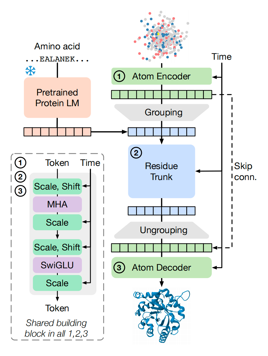
SimpleFold 的架构(上图所示)包含三个主要模块,并遵循“细粒度-粗粒度-细粒度”(“fine - coarse - fine”)的方案来实现蛋白质的层次化结构(hierarchical structure),以平衡性能和效率。
以下是对 SimpleFold 结构及其主要模块的解释:
1. 核心构建块:带自适应层的标准 Transformer 模块
SimpleFold 的所有模块(原子编码器、残基主干和原子解码器)都采用带自适应层(adaptive layers)的标准 Transformer 块来实现。这种带自适应层的 Transformer 块是 SimpleFold 共享的构建块。
- 时间步长 的条件化(Conditioning on Timestep ): 这些 Transformer 块通过 Adaptive Layers (AdaLN) 对时间步长 进行条件化处理。时间步长 的信息(Time Token)通过 Scale 和 Shift 操作被整合到 Transformer 块中。
- 组件(Shared Building Block): 每个共享构建块通常包括多头注意力(MHA)和 SwiGLU(一种替代标准前馈网络 FFN 的实现)。
2. 三个主要模块
SimpleFold 架构的流程始于输入氨基酸序列 和带有噪声的原子坐标 ,最终输出预测的速度场 。
(1) 预训练蛋白质语言模型(Pretrained Protein LM)
- 功能: SimpleFold 使用冻结的预训练蛋白质语言模型(PLM)(如 ESM2-3B)将氨基酸序列 嵌入到信息丰富的潜在表示 中。
- 作用: 这个嵌入 充当了生成模型的“文本提示”(类似于视觉生成模型中的文本提示),用于条件化地生成蛋白质结构。
(2) 原子编码器(Atom Encoder)
- 输入: 原子编码器接收带有噪声的原子坐标 (, 是重原子数)以及对应的原子特征(如原子类型和电荷)作为输入。
- 编码方式: 通过 Fourier 位置嵌入进行编码。
- 输出: 原子编码器输出原子 Token 。
- 局部注意力: 在原子编码器中,采用局部注意力掩码(local attention mask),将原子潜在表示限制为只关注其所在残基周围的局部邻域(即原子 Token 只关注序列中附近残基的原子 Token)。
(3) 残基主干(Residue Trunk)
- “分组”(Grouping)操作: 这是从细粒度(原子)到粗粒度(残基)的转换。分组操作对同一残基内的原子 Token 进行平均池化(average pooling),从而获得残基 Token ( 是残基数)。
- 输入: 残基 Token 与来自 PLM 的序列嵌入 沿通道维度进行拼接,然后输入到残基主干。
- 参数和计算量: 残基主干包含了模型大部分的参数,并且是大部分计算发生的地方。
(4) 原子解码器(Atom Decoder)
- “解分组”(Ungrouping)操作: 这是从粗粒度(残基)到细粒度(原子)的转换。解分组操作将更新后的残基 Token 投射到相应的原子 Token 上。具体来说,同一个残基 Token 会被复制(replicate)到该残基包含的所有原子上。
- 跳跃连接(Skip Connection): 原子编码器的输出通过跳跃连接(Skip conn.)也被添加到解码器,用于区分同一残基内的不同原子。
- 更新与输出: 原子解码器更新原子 Token,并最终输出预测的速度场 。
- 局部注意力: 原子解码器中也应用了局部注意力掩码,与编码器类似。
3. SimpleFold 架构的关键特点总结
SimpleFold 架构的设计旨在摆脱 AlphaFold2 等模型的复杂性,证明了仅使用通用架构也能实现强大的蛋白质折叠性能。
- 通用性: SimpleFold 仅基于通用 Transformer 模块,没有使用昂贵的、特定领域的设计,如多序列比对(MSA)、显式配对表示或三角更新。
- 效率: 由于只保留了单一的序列表示,SimpleFold 不需要三角更新,因此在计算上更为高效。例如,SimpleFold-3B 的前向计算量()远低于 AlphaFold2(),即使两者的参数量接近。
- 层次结构: 模型实现了“细粒度-粗粒度-细粒度”(原子 残基 原子)的方案来处理蛋白质的层次化结构。
- 位置编码: 模型在残基主干中使用了旋转位置嵌入(RoPE)。在原子编码器和解码器中,使用了轴向 4D RoPE 来编码原子和残基的位置信息。
- 等变性处理: SimpleFold 建基于标准的非等变 Transformer 块,为了处理蛋白质结构的旋转对称性,它在训练过程中应用了 SO(3) 数据增强(随机旋转结构目标),并依赖模型容量直接从数据中学习这些对称性。
结果如何?
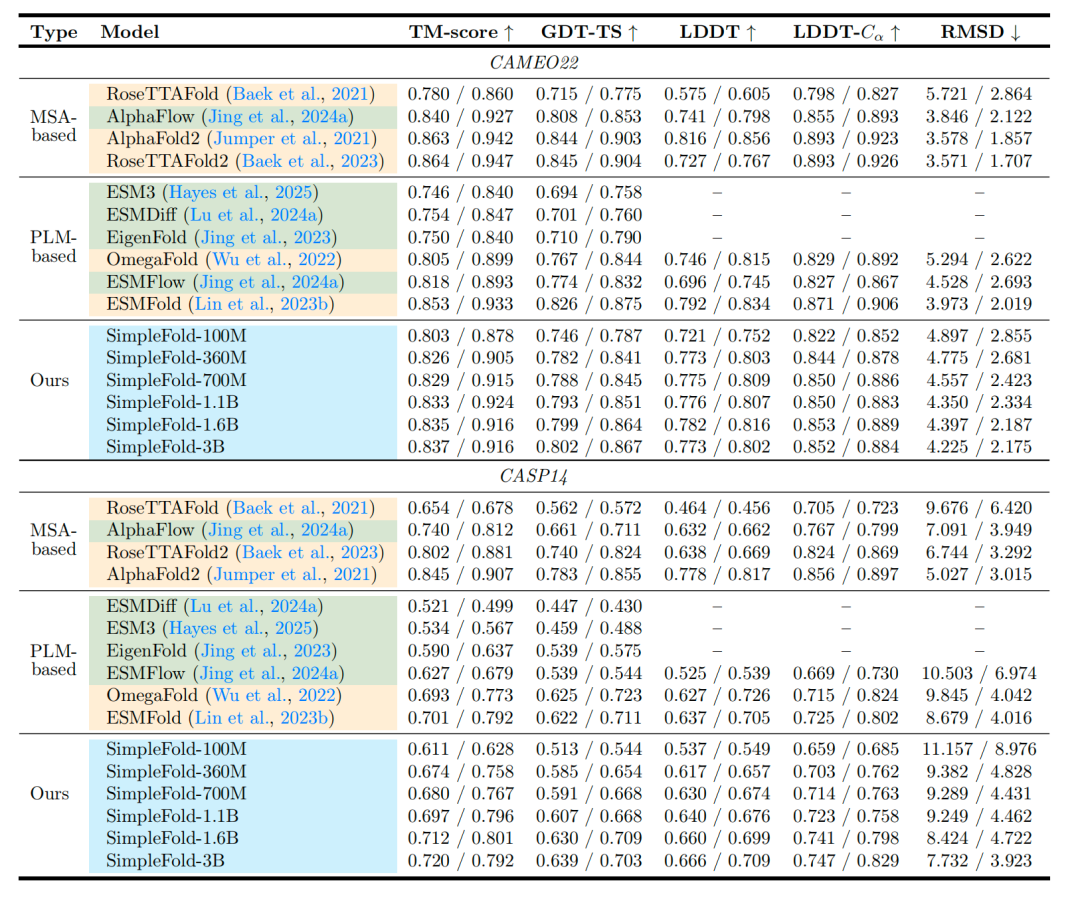
可以发现simlefold一共有6个版本,和其他模型在cameo22和casp14数据集上进行测试,可以发现,simplefold各版本的tm-score均超越了现有模型的性能,图中还列出了其他指标的比较,读者可自行阅读。
二.使用SimpleFold进行蛋白质结构预测
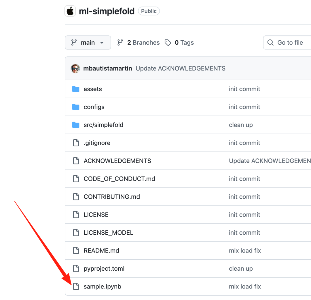
首先介绍一下simpleFold的官方地址:
https://github.com/apple/ml-simplefold
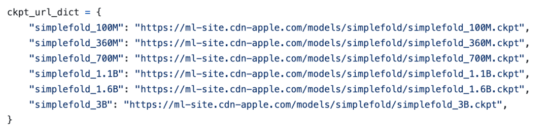
然后是SimpleFold的其他版本的权重下载地址:
2.1安装
git clone https://github.com/apple/ml-simplefold.git
cd ml-simplefold
conda create -n simplefold python=3.10
python -m pip install -U pip build; pip install -e .
安装官方的指令下载程序和安装依赖
然后打开sample.ipynb
开始进行蛋白质结构预测:
依赖:
import sys
import numpy as np
from math import pow
import py3Dmol
from pathlib import Path
from io import StringIO
from Bio.PDB import PDBIO
from Bio.PDB import MMCIFParser, Superimposer
sys.path.append(str(Path("./src/simplefold").resolve()))
输入一些序列,使用7ftv_A序列进行结构预测:
# following are example amino acid sequences:
example_sequences = {
    "7ftv_A": "GASKLRAVLEKLKLSRDDISTAAGMVKGVVDHLLLRLKCDSAFRGVGLLNTGSYYEHVKISAPNEFDVMFKLEVPRIQLEEYSNTRAYYFVKFKRNPKENPLSQFLEGEILSASKMLSKFRKIIKEEINDDTDVIMKRKRGGSPAVTLLISEKISVDITLALESKSSWPASTQEGLRIQNWLSAKVRKQLRLKPFYLVPKHAEETWRLSFSHIEKEILNNHGKSKTCCENKEEKCCRKDCLKLMKYLLEQLKERFKDKKHLDKFSSYHVKTAFFHVCTQNPQDSQWDRKDLGLCFDNCVTYFLQCLRTEKLENYFIPEFNLFSSNLIDKRSKEFLTKQIEYERNNEFPVFD",
    "8cny_A": "MGPSLDFALSLLRRNIRQVQTDQGHFTMLGVRDRLAVLPRHSQPGKTIWVEHKLINILDAVELVDEQGVNLELTLVTLDTNEKFRDITKFIPENISAASDATLVINTEHMPSMFVPVGDVVQYGFLNLSGKPTHRTMMYNFPTKAGQCGGVVTSVGKVIGIHIGGNGRQGFCAGLKRSYFAS",
    "8g8r_A": "GTVNWSVEDIVKGINSNNLESQLQATQAARKLLSREKQPPIDNIIRAGLIPKFVSFLGKTDCSPIQFESAWALTNIASGTSEQTKAVVDGGAIPAFISLLASPHAHISEQAVWALGNIAGDGSAFRDLVIKHGAIDPLLALLAVPDLSTLACGYLRNLTWTLSNLCRNKNPAPPLDAVEQILPTLVRLLHHNDPEVLADSCWAISYLTDGPNERIEMVVKKGVVPQLVKLLGATELPIVTPALRAIGNIVTGTDEQTQKVIDAGALAVFPSLLTNPKTNIQKEATWTMSNITAGRQDQIQQVVNHGLVPFLVGVLSKADFKTQKEAAWAITNYTSGGTVEQIVYLVHCGIIEPLMNLLSAKDTKIIQVILDAISNIFQAAEKLGETEKLSIMIEECGGLDKIEALQRHENESVYKASLNLIEKYFS",
    "8i85_A": "MGILQANRVLLSRLLPGVEPEGLTVRHGQFHQVVIASDRVVCLPRTAAAAARLPRRAAVMRVLAGLDLGCRTPRPLCEGSLPFLVLSRVPGAPLEADALEDSKVAEVVAAQYVTLLSGLASAGADEKVRAALPAPQGRWRQFAADVRAELFPLMSDGGCRQAERELAALDSLPDITEAVVHGNLGAENVLWVRDDGLPRLSGVIDWDEVSIGDPAEDLAAIGAGYGKDFLDQVLTLGGWSDRRMATRIATIRATFALQQALSACRDGDEEELADGLTGYR",
    "8g8r_A_x": "GTVNWSVEDIVKGINSNNLESQLQATQAARKLLSREKQPPIDNIIRAGLIPKFVSFLGKTDCSPIQFESAWALTNIASGTSEQTKAVVDGGAIPAFISLLASPHAHISEQAVWALGNIAGDGSAFRDLVIKHGAIDPLLALLAVPDLSTLACGYLRNLTWTLSNLCRNKNPAPPLDAVEQILPTLVRLLHHNDPEVLADSCWAISYLTDGPNERIEMVVKKGVVPQLVKLLGATELPIVTPALRAIGNIVTGTDEQTQKVIDAGALAVFPSLLTNPKTNIQKEATWTMSNITAGRQDQIQQVVNHGLVPFLVGVLSKADFKTQKEAAWAITNYTSGGTVEQIVYLVHCGIIEPLMNLLSAKDTKIIQVILDAISNIFQAAEKLGETEKLSIMIEECGGLDKIEALQRHENESVYKASLNLIEKYFSGTVNWSVEDIVKGINSNNLESQLQATQAARKLLSREKQPPIDNIIRAGLIPKFVSFLGKTDCSPIQFESAWALTNIASGTSEQTKAVVDGGAIPAFISLLASPHAHISEQAVWALGNIAGDGSAFRDLVIKHGAIDPLLALLAVPDLSTLACGYLRNLTWTLSNLCRNKNPAPPLDAVEQILPTLVRLLHHNDPEVLADSCWAISYLTDGPNERIEMVVKKGVVPQLVKLLGATELPIVTPALRAIGNIVTGTDEQTQKVIDAGALAVFPSLLTNPKTNIQKEATWTMSNITAGRQDQIQQVVNHGLVPFLVGVLSKADFKTQKEAAWAITNYTSGGTVEQIVYLVHCGIIEPLMNLLSAKDTKIIQVILDAISNIFQAAEKLGETEKLSIMIEECGGLDKIEALQRHENESVYKASLNLIEKYFSISEQAVWALGNIAGDGSAFRDLVIKHGAIDPLLALLAVPDLSTLACGYLRNLTWTLSNLCRNKNPAPPLDAVEQILPTLVRLLHHNDPEVLADSCWAISYLTDGPNERIEMVVKKGVVPQLVKLLGATELPIVTPALRAIGNIVTGTDEQTQKVIDAGALAVFPSLLTNPKTNIQKEATWTMSNITAGRQDQIQQVVNHGLVPFLVGVLSKADFKTQKEAAWAITNYTSGGTVEQIVYLVHCGIIEPLMNLLSAKDTKIIQVILDAISNIFQAAEKLGETEKLSIMIEECGGLDKIEALQRHENESVYKASLNLIEKYFSGTVNWSVEDIVKGINSNNLESQLQATQAARKLLSREKQPPIDNIIRAGLIPKFVSFLGKTDCSPIQFESAWALTNIASGTSEQTKAVVDGGAIPAFISLLASPHAHISEQAVWALGNIAGDGSAFRDLVIKHGAIDPLLALLAVPDLSTLACGYLRNLTWTLSNLCRNKNPAPPLDAVEQILPTLVRLLHHNDPEVLADSCWAISYLTDGPNERIEMVVKKGVVPQLVKLLGATELPIVTPALRAIGNIVTGTDEQTQKVIDAGALAVFPSLLTNPKTNIQKEATWTMSNITAGRQDQIQQVVNHGLVPFLVGVLSKADFKTQKEAAWAITNYTSGGTVEQIVYLVHCGIIEPLMNLLSAKDTKIIQVILDAISNIFQAAEKLGETEKLSIMIEECGGLDKIEALQRHENESVYKASLNLIEKYFS",
}
seq_id = "7ftv_A"  # choose from example_sequences
aa_sequence = example_sequences[seq_id]
print(f"Predicting structure for {seq_id} with {len(aa_sequence)} amino acids.")
指定参数:
simplefold_model = "simplefold_3B" # choose from 100M, 360M, 700M, 1.1B, 1.6B, 3B
backend = "mlx" # choose from ["mlx", "torch"]
ckpt_dir = "artifacts"
output_dir = "artifacts"
prediction_dir = f"predictions_{simplefold_model}_{backend}"
output_name = f"{seq_id}"
num_steps = 500 # number of inference steps for flow-matching
tau = 0.05 # stochasticity scale
plddt = True # whether to use pLDDT confidence module
nsample_per_protein = 1 # number of samples per protein
simpleFold目前一共有6个模型
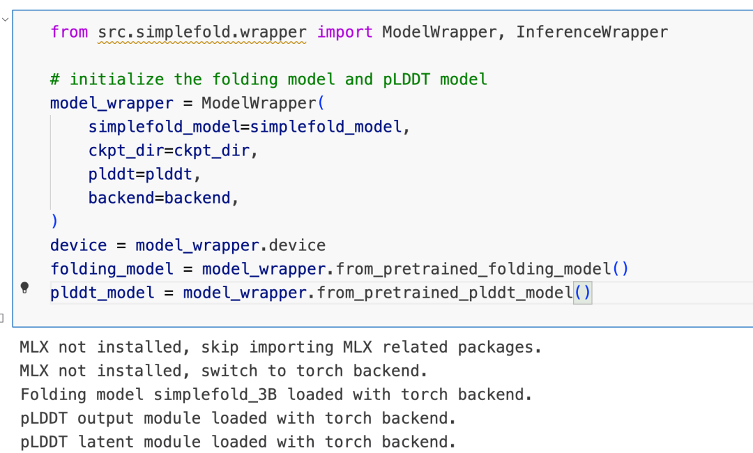
下一步,初始化加载器:
from src.simplefold.wrapper import ModelWrapper, InferenceWrapper
# initialize the folding model and pLDDT model
model_wrapper = ModelWrapper(
    simplefold_model=simplefold_model,
    ckpt_dir=ckpt_dir,
    plddt=plddt,
    backend=backend,
)
device = model_wrapper.device
folding_model = model_wrapper.from_pretrained_folding_model()
plddt_model = model_wrapper.from_pretrained_plddt_model()
这一步,需要下载很多文件,有几个坑,可以和大家share一下:
首先这是一张加载成功的输出:
第一,这个模型会首先会下载 simpleFold_3b这个模型,如果服务器的网络不行,则可以手动Magic然后进行下载:
https://ml-site.cdn-apple.com/models/simplefold/simplefold_3B.ckpt第二,模型使用plddt作为打分函数,所以需要下载plddt的权重进行直接预测,遇到同样的网络问题需要大家手动Magic进行下载:
https://ml-site.cdn-apple.com/models/simplefold/plddt_module_1.6B.ckpt接下来,继续加载蛋白质语言模型(esm-3b)提取蛋白质的特征向量,
# initialize the inference module with inference configurations
inference_wrapper = InferenceWrapper(
    output_dir=output_dir,
    prediction_dir=prediction_dir,
    num_steps=num_steps,
    tau=tau,
    nsample_per_protein=nsample_per_protein,
    device=device,
    backend=backend
)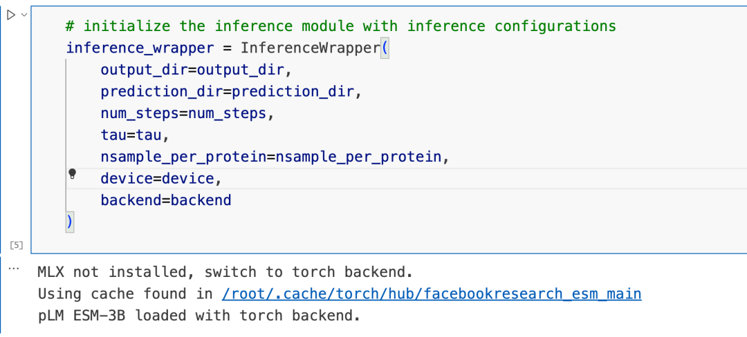
这一步,模型会下载esm-3b这个esm2家族中最小的模型进行蛋白质序列特征提取,并且还会下载ccd.pkl文件,这个文件会因为网络问题无法下载,所以汤姆手动找到了一个下载地址:
https://boltz1.s3.us-east-2.amazonaws.com/ccd.pkl这个文件包含了模型所需要的原子特征和构象数据。
第二,由于SimpleFold的数据处理步骤用到了blotz中的一些过程,所以需要下载一个很大的boltz权重文件,3.6G,同样在服务器上进行下载的时候会遇到下载失败的问题,所以下面是可直接下载的链接:
https://huggingface.co/boltz-community/boltz-1/resolve/refs%2Fpr%2F8/boltz1_conf.ckpt第三个是esm-3b的下载地址,这个大家自行解决即可。
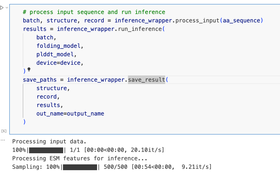
接下来就是开始预测序列的结构:
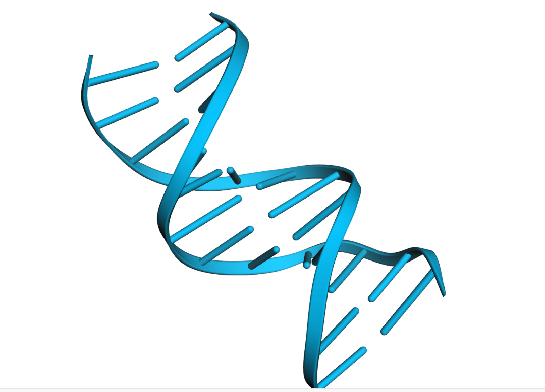
可视化结果:
# visualize the first predicted structure
pdb_path = save_paths[0]
view = py3Dmol.view(query=pdb_path)# color based on the predicted confidence
# confidence coloring from low to high: red–orange–yellow–green–blue (0 to 100)
if plddt:
view.setStyle({'cartoon':{'colorscheme':{'prop':'b','gradient':'roygb','min':0,'max':100}}})
view.zoomTo()
view.show()
# color in spectrum if pLDDT is not available
else:
view.setStyle({'cartoon':{'color':'spectrum'}})
view.zoomTo()
view.show()输出:
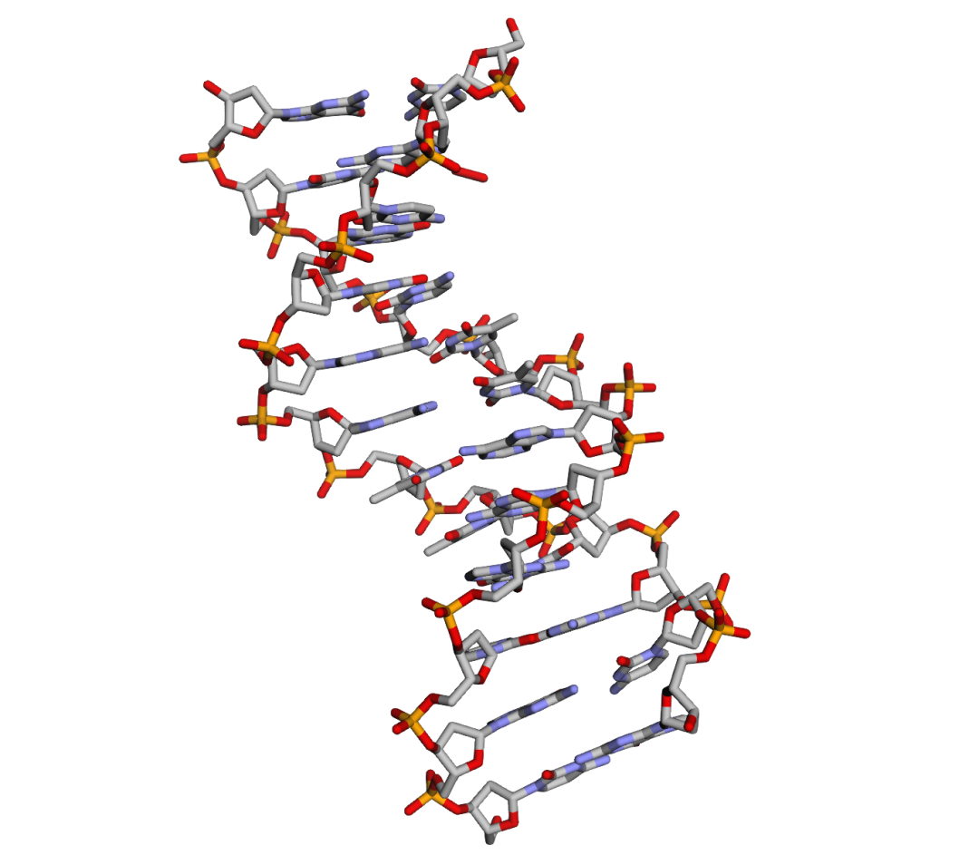
查看所有原子的结构:
# visualize the all-atom structure
view.setStyle({'stick':{}})
view.zoomTo()
view.show()
输出:
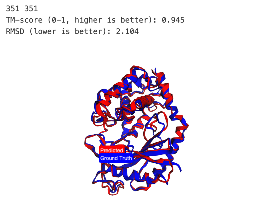
指标计算(official edition):
# visualize the predicted structure in 3D alongside the GT structure
def calculate_tm_score(coords1, coords2, L_target=None):
    """
    Compute TM-score for two aligned coordinate sets (numpy arrays).

    coords1, coords2: Nx3 numpy arrays (aligned atomic coordinates, e.g. CA atoms)
    L_target: length of target protein (default = len(coords1))
    """
    assert coords1.shape == coords2.shape, "Aligned coords must have same shape"
    N = coords1.shape[0]
    if L_target is None:
        L_target = N
    # distances between aligned atoms
    dists = np.linalg.norm(coords1 - coords2, axis=1)
    # scaling factor d0
    d0 = 1.24 * pow(L_target - 15, 1/3) - 1.8
    if d0 < 0.5:
        d0 = 0.5  # safeguard, as in TM-align
    # TM-score
    score = np.sum(1.0 / (1.0 + (dists/d0)**2)) / L_target
    return score
parser = MMCIFParser(QUIET=True)
# Load two structures
struct1 = parser.get_structure("ref", f"assets/{seq_id}.cif")
struct2 = parser.get_structure("prd", pdb_path)
# Select CA atoms for alignment
atoms1 = [a for a in struct1.get_atoms() if a.get_id() == 'CA']
atoms2 = [a for a in struct2.get_atoms() if a.get_id() == 'CA']
print(len(atoms1), len(atoms2))
# Superimpose
sup = Superimposer()
sup.set_atoms(atoms1, atoms2)
sup.apply(struct2.get_atoms())
# Calculate TM-score
coords1 = np.array([a.coord for a in atoms1])
coords2 = np.array([a.coord for a in atoms2])
tm_score = calculate_tm_score(coords1, coords2)
print("TM-score (0-1, higher is better): {:.3f}".format(tm_score))
print("RMSD (lower is better): {:.3f}".format(sup.rms))
# Save aligned structures to strings
io = PDBIO()
s1_buf, s2_buf = StringIO(), StringIO()
io.set_structure(struct1); io.save(s1_buf)
io.set_structure(struct2); io.save(s2_buf)
# Visualize in py3Dmol
view = py3Dmol.view(width=600, height=400)
view.addModel(s1_buf.getvalue(),"pdb")
view.addModel(s2_buf.getvalue(),"pdb")
# Color reference protein blue, predicted structure red
view.setStyle({'model': 0}, {'cartoon': {'color': 'blue'}})
view.setStyle({'model': 1}, {'cartoon': {'color': 'red'}})
# Add legend
view.addLabel("Ground Truth", {'position': {'x': 0, 'y': 0, 'z': 0}, 'backgroundColor': 'blue', 'fontColor': 'white', 'fontSize': 12})
view.addLabel("Predicted", {'position': {'x': 0, 'y': 4, 'z': 0}, 'backgroundColor': 'red', 'fontColor': 'white', 'fontSize': 12})
view.zoomTo()
view.show()
输出:
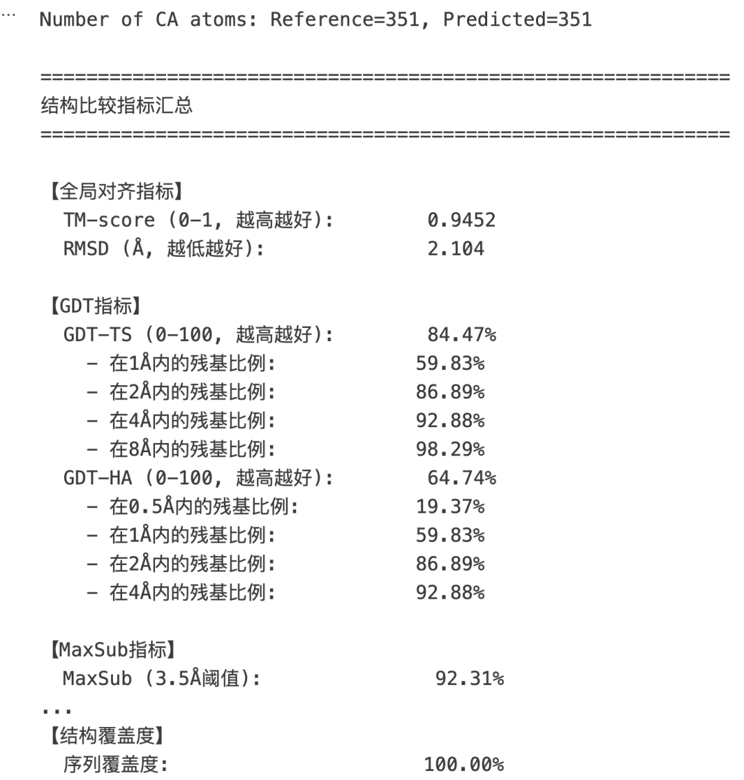
除了官方版本的指标计算,汤姆还写了一个多指标计算的脚本:
import numpy as np
from Bio.PDB import MMCIFParser, Superimposer, PDBIO
from scipy.spatial.distance import cdist
import py3Dmol
from io import StringIO
# ===================== 原有指标 =====================
def calculate_tm_score(coords1, coords2, L_target=None):
    """
    Compute TM-score for two aligned coordinate sets (numpy arrays).

    coords1, coords2: Nx3 numpy arrays (aligned atomic coordinates, e.g. CA atoms)
    L_target: length of target protein (default = len(coords1))
    """
    assert coords1.shape == coords2.shape, "Aligned coords must have same shape"
    N = coords1.shape[0]
    if L_target is None:
        L_target = N
    # distances between aligned atoms
    dists = np.linalg.norm(coords1 - coords2, axis=1)
    # scaling factor d0
    d0 = 1.24 * pow(L_target - 15, 1/3) - 1.8
    if d0 < 0.5:
        d0 = 0.5  # safeguard, as in TM-align
    # TM-score
    score = np.sum(1.0 / (1.0 + (dists/d0)**2)) / L_target
    return score
# ===================== 新增指标 =====================
def calculate_gdt_ts(coords1, coords2, cutoffs=[1.0, 2.0, 4.0, 8.0]):
    """
    Global Distance Test - Total Score (GDT-TS)
    计算在不同距离阈值下正确对齐的原子百分比的平均值

    常用于CASP蛋白质结构预测评估
    """
    assert coords1.shape == coords2.shape
    N = coords1.shape[0]
    dists = np.linalg.norm(coords1 - coords2, axis=1)

    percentages = []
    for cutoff in cutoffs:
        percent = np.sum(dists < cutoff) / N * 100
        percentages.append(percent)

    gdt_ts = np.mean(percentages)
    return gdt_ts, percentages
def calculate_gdt_ha(coords1, coords2, cutoffs=[0.5, 1.0, 2.0, 4.0]):
    """
    Global Distance Test - High Accuracy (GDT-HA)
    使用更严格的阈值,适合高精度结构比较
    """
    return calculate_gdt_ts(coords1, coords2, cutoffs)
def calculate_maxsub_score(coords1, coords2, threshold=3.5):
    """
    MaxSub Score: 在给定阈值下最大对齐子集的百分比
    """
    assert coords1.shape == coords2.shape
    N = coords1.shape[0]
    dists = np.linalg.norm(coords1 - coords2, axis=1)
    maxsub = np.sum(dists < threshold) / N * 100
    return maxsub
def calculate_lddt(coords1, coords2, all_coords1=None, all_coords2=None,
                   cutoffs=[0.5, 1.0, 2.0, 4.0], inclusion_radius=15.0):
    """
    Local Distance Difference Test (lDDT)
    评估局部距离保留情况,不需要全局对齐

    all_coords1, all_coords2: 如果提供,用于计算更精确的局部环境
    """
    if all_coords1 is None:
        all_coords1 = coords1
    if all_coords2 is None:
        all_coords2 = coords2

    N = coords1.shape[0]
    preserved_contacts = 0
    total_contacts = 0

    for i in range(N):
        # 计算参考结构中的局部距离
        ref_dists = np.linalg.norm(all_coords1[i] - all_coords1, axis=1)
        local_mask = (ref_dists > 0) & (ref_dists < inclusion_radius)

        if not np.any(local_mask):
            continue

        # 计算预测结构中的对应距离
        pred_dists = np.linalg.norm(all_coords2[i] - all_coords2, axis=1)

        # 对于每个局部接触,检查距离差异
        for cutoff in cutoffs:
            diff = np.abs(ref_dists[local_mask] - pred_dists[local_mask])
            preserved_contacts += np.sum(diff < cutoff)
            total_contacts += np.sum(local_mask) * len(cutoffs)

    lddt_score = preserved_contacts / total_contacts if total_contacts > 0 else 0
    return lddt_score * 100  # 返回百分比
def calculate_contact_overlap(coords1, coords2, distance_threshold=8.0):
    """
    接触图重叠度:计算两个结构中距离<阈值的残基对的重叠比例
    """
    # 计算距离矩阵
    dist_mat1 = cdist(coords1, coords1)
    dist_mat2 = cdist(coords2, coords2)

    # 定义接触
    contacts1 = (dist_mat1 < distance_threshold) & (dist_mat1 > 0)
    contacts2 = (dist_mat2 < distance_threshold) & (dist_mat2 > 0)

    # 计算重叠
    overlap = np.sum(contacts1 & contacts2)
    union = np.sum(contacts1 | contacts2)

    if union == 0:
        return 0.0

    return overlap / union * 100
def calculate_dihedral_angles(coords):
    """
    计算骨架二面角 (phi, psi)
    需要连续的CA坐标
    """
    angles = []
    for i in range(1, len(coords) - 1):
        # 简化版本:仅基于CA坐标估算
        v1 = coords[i] - coords[i-1]
        v2 = coords[i+1] - coords[i]

        # 计算角度
        cos_angle = np.dot(v1, v2) / (np.linalg.norm(v1) * np.linalg.norm(v2))
        angle = np.arccos(np.clip(cos_angle, -1.0, 1.0))
        angles.append(np.degrees(angle))

    return np.array(angles)
def calculate_dihedral_similarity(coords1, coords2):
    """
    比较两个结构的二面角相似性
    """
    angles1 = calculate_dihedral_angles(coords1)
    angles2 = calculate_dihedral_angles(coords2)

    if len(angles1) != len(angles2):
        return None

    # 计算角度差异的平均值
    angle_diff = np.abs(angles1 - angles2)
    # 处理周期性 (0-360度)
    angle_diff = np.minimum(angle_diff, 360 - angle_diff)

    mean_diff = np.mean(angle_diff)
    return mean_diff
def calculate_per_residue_rmsd(coords1, coords2):
    """
    计算每个残基的RMSD,用于识别哪些区域差异较大
    """
    per_res_rmsd = np.linalg.norm(coords1 - coords2, axis=1)
    return per_res_rmsd
def calculate_radius_of_gyration(coords):
    """
    回转半径:衡量蛋白质的紧凑程度
    """
    center = np.mean(coords, axis=0)
    rg = np.sqrt(np.mean(np.sum((coords - center)**2, axis=1)))
    return rg
def calculate_structure_compactness_difference(coords1, coords2):
    """
    比较两个结构的紧凑程度差异
    """
    rg1 = calculate_radius_of_gyration(coords1)
    rg2 = calculate_radius_of_gyration(coords2)
    return abs(rg1 - rg2), rg1, rg2
def calculate_coverage(coords1, coords2):
    """
    计算结构覆盖度(对齐的残基比例)
    """
    return min(len(coords1), len(coords2)) / max(len(coords1), len(coords2)) * 100
# ===================== 主程序 =====================
parser = MMCIFParser(QUIET=True)
# Load two structures
struct1 = parser.get_structure("ref", f"assets/{seq_id}.cif")
struct2 = parser.get_structure("prd", pdb_path)
# Select CA atoms for alignment
atoms1 = [a for a in struct1.get_atoms() if a.get_id() == 'CA']
atoms2 = [a for a in struct2.get_atoms() if a.get_id() == 'CA']
print(f"Number of CA atoms: Reference={len(atoms1)}, Predicted={len(atoms2)}")
# Superimpose
sup = Superimposer()
sup.set_atoms(atoms1, atoms2)
sup.apply(struct2.get_atoms())
# Get coordinates
coords1 = np.array([a.coord for a in atoms1])
coords2 = np.array([a.coord for a in atoms2])
# ===================== 计算所有指标 =====================
print("\n" + "="*60)
print("结构比较指标汇总")
print("="*60)
# 1. 原有指标
tm_score = calculate_tm_score(coords1, coords2)
rmsd = sup.rms
print(f"\n【全局对齐指标】")
print(f"  TM-score (0-1, 越高越好):        {tm_score:.4f}")
print(f"  RMSD (Å, 越低越好):              {rmsd:.3f}")
# 2. GDT-TS 和 GDT-HA
gdt_ts, gdt_ts_percentages = calculate_gdt_ts(coords1, coords2)
gdt_ha, gdt_ha_percentages = calculate_gdt_ha(coords1, coords2)
print(f"\n【GDT指标】")
print(f"  GDT-TS (0-100, 越高越好):        {gdt_ts:.2f}%")
print(f"    - 在1Å内的残基比例:            {gdt_ts_percentages[0]:.2f}%")
print(f"    - 在2Å内的残基比例:            {gdt_ts_percentages[1]:.2f}%")
print(f"    - 在4Å内的残基比例:            {gdt_ts_percentages[2]:.2f}%")
print(f"    - 在8Å内的残基比例:            {gdt_ts_percentages[3]:.2f}%")
print(f"  GDT-HA (0-100, 越高越好):        {gdt_ha:.2f}%")
print(f"    - 在0.5Å内的残基比例:          {gdt_ha_percentages[0]:.2f}%")
print(f"    - 在1Å内的残基比例:            {gdt_ha_percentages[1]:.2f}%")
print(f"    - 在2Å内的残基比例:            {gdt_ha_percentages[2]:.2f}%")
print(f"    - 在4Å内的残基比例:            {gdt_ha_percentages[3]:.2f}%")
# 3. MaxSub
maxsub = calculate_maxsub_score(coords1, coords2)
print(f"\n【MaxSub指标】")
print(f"  MaxSub (3.5Å阈值):               {maxsub:.2f}%")
# 4. lDDT
lddt = calculate_lddt(coords1, coords2)
print(f"\n【局部距离保留】")
print(f"  lDDT (0-100, 越高越好):          {lddt:.2f}%")
# 5. 接触图重叠
contact_overlap = calculate_contact_overlap(coords1, coords2)
print(f"\n【接触图分析】")
print(f"  接触重叠度 (8Å阈值):            {contact_overlap:.2f}%")
# 6. 二面角相似性
dihedral_sim = calculate_dihedral_similarity(coords1, coords2)
if dihedral_sim is not None:
    print(f"\n【二面角分析】")
    print(f"  平均二面角差异 (度):            {dihedral_sim:.2f}°")
# 7. 结构紧凑度
rg_diff, rg1, rg2 = calculate_structure_compactness_difference(coords1, coords2)
print(f"\n【结构紧凑度】")
print(f"  参考结构回转半径 (Å):           {rg1:.3f}")
print(f"  预测结构回转半径 (Å):           {rg2:.3f}")
print(f"  回转半径差异 (Å):               {rg_diff:.3f}")
# 8. 每残基RMSD分析
per_res_rmsd = calculate_per_residue_rmsd(coords1, coords2)
print(f"\n【每残基分析】")
print(f"  平均每残基RMSD (Å):             {np.mean(per_res_rmsd):.3f}")
print(f"  最大每残基RMSD (Å):             {np.max(per_res_rmsd):.3f}")
print(f"  RMSD标准差 (Å):                 {np.std(per_res_rmsd):.3f}")
print(f"  >5Å偏差的残基数:                {np.sum(per_res_rmsd > 5)}")
# 9. 覆盖度
coverage = calculate_coverage(coords1, coords2)
print(f"\n【结构覆盖度】")
print(f"  序列覆盖度:                      {coverage:.2f}%")
print("\n" + "="*60)
# ===================== 可视化 =====================
# Save aligned structures to strings
io = PDBIO()
s1_buf, s2_buf = StringIO(), StringIO()
io.set_structure(struct1); io.save(s1_buf)
io.set_structure(struct2); io.save(s2_buf)
# Visualize in py3Dmol with per-residue coloring
view = py3Dmol.view(width=800, height=500)
view.addModel(s1_buf.getvalue(),"pdb")
view.addModel(s2_buf.getvalue(),"pdb")
# Color by per-residue RMSD (optional advanced visualization)
view.setStyle({'model': 0}, {'cartoon': {'color': 'blue', 'opacity': 0.7}})
view.setStyle({'model': 1}, {'cartoon': {'color': 'red', 'opacity': 0.7}})
# Add legend
view.addLabel("Ground Truth", {'position': {'x': 0, 'y': 0, 'z': 0},
              'backgroundColor': 'blue', 'fontColor': 'white', 'fontSize': 12})
view.addLabel("Predicted", {'position': {'x': 0, 'y': 4, 'z': 0},
              'backgroundColor': 'red', 'fontColor': 'white', 'fontSize': 12})
view.zoomTo()
view.show()
# ===================== 可选:保存详细报告 =====================
# 保存每残基RMSD到文件,用于进一步分析
np.savetxt('per_residue_rmsd.txt', per_res_rmsd,
           header='Per-residue RMSD (Angstrom)', fmt='%.3f')
输出:
最后的最后,汤姆也使用alphafold3进行了同样序列的结构预测:
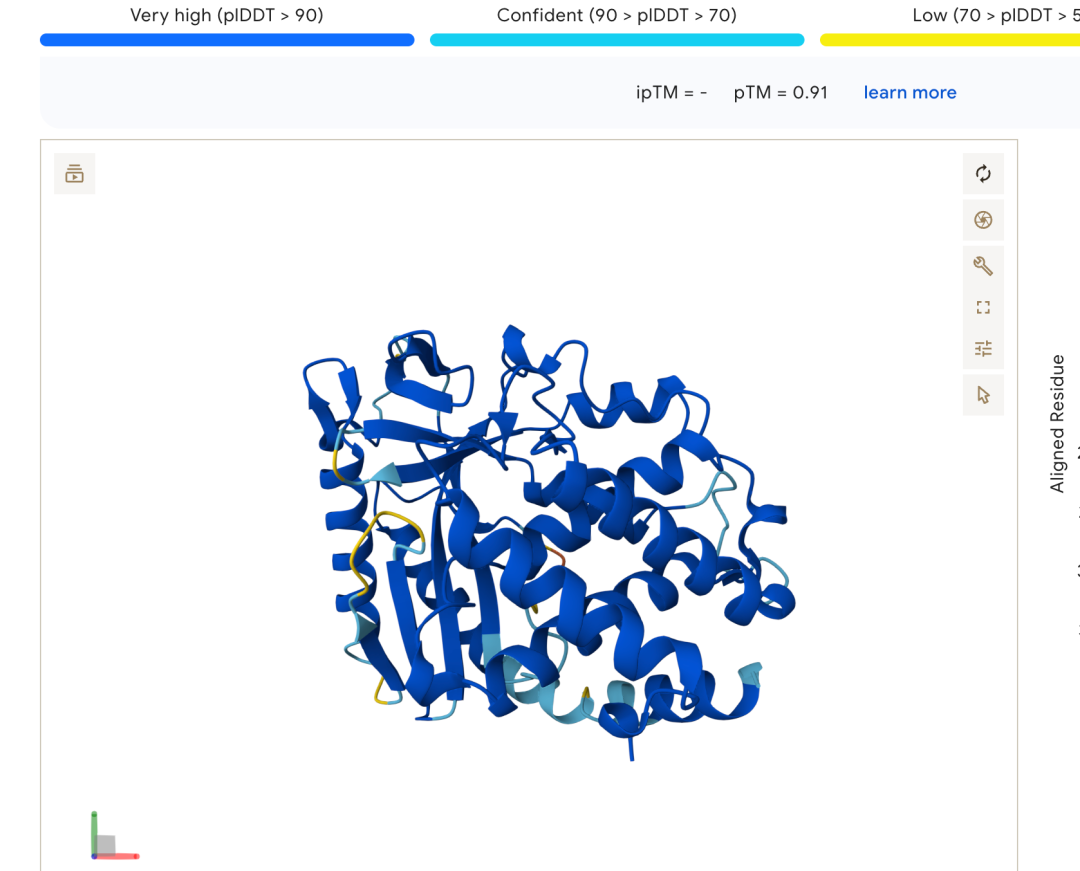
tm值只有0.91 ,速度的话,大概是大于60s,使用simplefold只用了54秒,但是 没有控制变量,所以无法衡量这两个大模型的预测速度,但是在simplefold的论文中,有这样一则图:
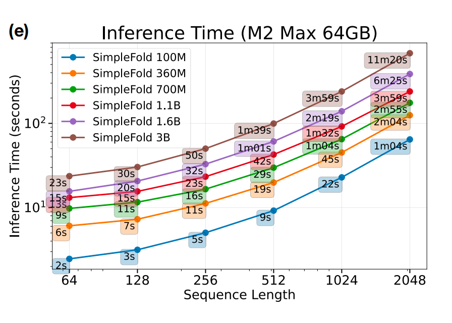
如果是这样子的话,在准确率比af3高的情况下,在Apple M2芯片上的预测速度还是可以的。
本次分享就到这里了,您的在看和点赞是我不断测试新模型,和不断调试的动力,谢谢大家。
本文参与 腾讯云自媒体同步曝光计划,分享自微信公众号。
原始发表:2025-10-06,如有侵权请联系 cloudcommunity@tencent.com 删除
评论
登录后参与评论
推荐阅读
目录
腾讯云开发者

Copyright © 2013 - 2026 Tencent Cloud. All Rights Reserved. 腾讯云 版权所有
深圳市腾讯计算机系统有限公司 ICP备案/许可证号:粤B2-20090059 ![]() 粤公网安备44030502008569号
粤公网安备44030502008569号
腾讯云计算(北京)有限责任公司 京ICP证150476号 | 京ICP备11018762号