构建AI智能体:Encoder-only与Decoder-only模型架构:基于本地小模型的实践解析
原创
构建AI智能体:Encoder-only与Decoder-only模型架构:基于本地小模型的实践解析
原创
未闻花名
发布于 2026-01-17 10:18:17
发布于 2026-01-17 10:18:17
一、前言
在大模型蓬勃发展的今天,我们天天被动输入,一度对这个名字都耳熟能详,但对于主流架构可能还没有接触的很深,大模型的Encoder-only与Decoder-only两大架构犹如两条截然不同的技术路径,也是我们需要关注深耕的,简单来说,Encoder-only模型如同一位深度分析师,它擅长一次性理解整段文本的完整含义,在情感分析、文本分类等理解型任务上表现卓越;而Decoder-only模型则更像一位创意写手,它通过自回归的方式逐词生成内容,在文本创作、对话系统等生成型场景中游刃有余。
这种技术路线的分层,直接映射到开发者面临的实际抉择:是专注于构建需要深度语义理解的企业应用,如智能客服、内容审核、知识问答系统?还是投身于需要创造性输出的产品开发,如智能写作助手、个性化对话机器人、代码生成工具?对于企业和个人开发者而言,这个选择远不止于技术偏好,更关系到产品方向、资源投入和职业发展路径。选择Encoder-only路线,意味着深耕自然语言理解领域,为企业提供精准的文本分析能力;选择Decoder-only路径,则是在内容生成的前沿阵地上开拓创新,为用户创造全新的交互体验。
今天我们将从实际应用出发,深入解析两种架构的特点,传统行业需要的不是华而不实的对话机器人,而是能够精准理解合同条款、快速分析客户反馈、智能识别风险信息的实用工具。这正是Encoder-only模型的用武之地,它如同一位经验丰富的分析师,能够透过文字表面,洞察深层含义。然而,市场同样渴求创新。内容创作、智能客服、代码生成等场景需要模型具备持续创作能力,这时候Decoder-only架构展现出独特价值。它就像不知疲倦的创作者,能够根据简单提示生成丰富内容。

二、Encoder-only 架构
1. 基础理解
对比我们的语文考试中阅读理解题目,好比我们阅读了一篇文章,然后进行分析后回答一些问题,Encoder-only 模型就是这样一位阅读理解大师。它的工作方式是:
- 一次性读取整段文本。
- 同时分析每一个字、每一个词与全文所有其他部分的关系。
- 为每个词生成一个包含了全文信息的深度理解版向量。
Encoder-only 模型像一个拥有超级大脑的读者,它拿到一篇文章后,不是从头读到尾,而是瞬间通览全文,深刻理解其内涵,为了让阅读理解成为可能,Encoder-only 模型的核心是一种叫做 “双向注意力机制” 的技术。
让我们用一个简单的例子来理解它:
- 句子:“苹果公司发布了新款手机。”
- 任务:理解“苹果”这个词在这里是什么意思。
我们通常的思考方式:
- 首先会看向“苹果”后面的词:“公司”、“发布”、“手机”。
- 通过这些上下文,我们会立刻明白,这里的“苹果”指的是科技公司,而不是一种水果。
Encoder-only 模型是思考方式:
- 模型会为句子中的每个词计算一个“注意力分数”,表示它应该多“关注”其他词。
- 对于 “苹果” 这个词,模型会计算出它与 “公司”、“发布”、“手机” 有很高的注意力分数。
- 同时,“公司” 这个词也会高度关注 “苹果”。
- “手机” 也会关注 “新款”、“发布” 和 “苹果”。
这个过程是同时发生的、双向的,就像一张所有词语相互连接的网络。
# 一个简化的注意力模式示意图 句子: [CLS] 苹果 公司 发布 了 新 手机 [SEP] 注意力模式 (所有词相互关注): [CLS] → 苹果, 公司, 发布, 了, 新, 手机, [SEP] 苹果 → [CLS], 公司, 发布, 了, 新, 手机, [SEP] 公司 → [CLS], 苹果, 发布, 了, 新, 手机, [SEP] 发布 → [CLS], 苹果, 公司, 了, 新, 手机, [SEP] ... (以此类推) 每个词都可以与句子中的所有其他词进行“交流”,获取全局信息。
2. 代表模型
BERT 是 Encoder-only 架构最著名的代表,它的出现彻底改变了自然语言处理领域,Encoder-only模型的预训练目标与生成式模型有本质不同,其核心是深度理解而非生成。
BERT 的训练过程,BERT 通过两个有趣的方式来学习语言:
进行“完形填空”(掩码语言模型 - MLM)
- 方法:随机遮盖出一句话中15%的词(例如,把“今天天气很好”变成“今天天气[MASK]”)。
- 任务:让模型根据上下文的所有词(包括后面的“好”),来预测被遮盖的词是什么。
- 这正是双向注意力的威力所在! 模型可以利用后半句的“好”来帮助预测前面的“[MASK]”是“很”。
直接“判断上下句”(下一句预测 - NSP)
- 方法:给模型两句话,让它判断第二句话是否是第一句话的下一句。
- 任务:帮助模型理解句子之间的关系,对于问答、推理任务至关重要。
通过海量文本上的这两种训练,BERT 学会了单词的深层含义、语法结构以及逻辑关系。
3. 核心架构
Encoder-only模型的核心是Transformer的编码器部分。要理解它,我们需要先回顾其核心工作机制:
1.1 自注意力机制:
- 核心功能:在处理一个词时,能够同时关注到输入序列中的所有其他词,并计算它们与当前词的相关性权重。
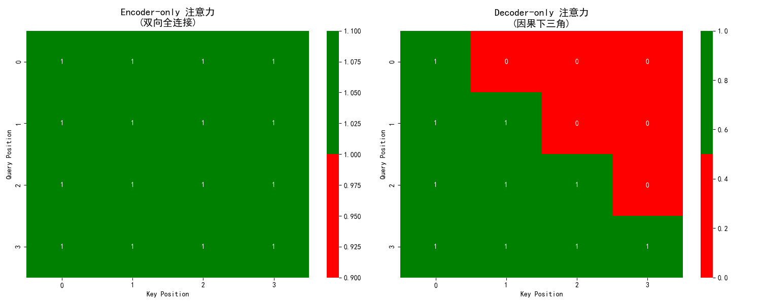
- 与Decoder的区别:Encoder使用的是双向自注意力,即每个词可以关注到其左侧和右侧的所有上下文信息。这使得它能深度、全面地理解整个句子的含义。
1.2 位置编码:
- 由于自注意力机制本身不包含顺序信息,需要通过位置编码为输入序列中的每个词注入其位置信息,使模型能够理解词的顺序。
1.3 前馈神经网络:
- 每个编码器层中的另一个核心组件,对自注意力层的输出进行非线性变换,增加模型的表达能力。
一个典型的Encoder-only模型(如BERT)由多层(例如12层、24层)上述结构堆叠而成。
4. 体现优势
双向上下文理解:
- 这是其最核心的优势。在理解任务中,一个词的含义往往由其前后文共同决定。Encoder-only架构能同时利用所有上下文信息,生成高质量的“上下文化词向量”。
擅长自然语言理解任务:
- 由于其强大的理解能力,它在各类NLU任务上表现极其出色,如文本分类、情感分析、命名实体识别、问答等。
对于理解任务非常高效:
- 在推理阶段,对于整个输入序列,只需进行一次前向传播即可得到所有词的表示,然后可以直接用于分类或标注等任务,计算效率很高。
5. 局限性
不擅长文本生成:
- 这是其最显著的短板。由于其双向注意力机制,在生成下一个词时,模型理论上可以“看到”未来的词,这会导致训练和推理的不一致。它没有像Decoder那样的自回归生成机制,因此无法进行流畅的、连续的文本生成。
计算开销(对长文本):
- 自注意力机制的计算复杂度与序列长度的平方成正比。处理非常长的文档时,计算和内存开销会非常大。
6. 应用场景
Encoder-only模型是典型的理解型模型,广泛应用于以下领域:
- 文本分类:主要用于情感分析、新闻分类、垃圾邮件检测,在序列的[CLS]标记输出上接一个分类器。
- 序列标注:进行命名实体识别、词性标注,对序列中的每一个词对应的输出向量进行分类。
- 语义相似度:针对语句进行重复问题识别、语义检索,比较两个句子编码向量的相似度,如余弦相似度。
- 问答系统:进行抽取式问答,根据问题和文章,预测答案在文章中的起始和结束位置。
- 自然语言推理:判断文本间的逻辑关系,判断两个句子是蕴含、矛盾还是中立关系。
7. 示例分析
7.1 句子对相似度比较
from transformers import BertTokenizer, BertForSequenceClassification
from modelscope import snapshot_download
import torch
from torch.nn.functional import cosine_similarity

# 1. 加载模型和分词器
cache_dir = "D:\\modelscope\\hub"
model_name = "google-bert/bert-base-chinese"
local_model_path = snapshot_download(model_name, cache_dir=cache_dir)
tokenizer = BertTokenizer.from_pretrained(local_model_path)
# 对于相似度任务,我们也可以使用专门为句向量优化的模型,如 sentence-transformers
# 这里我们用基础BERT演示获取句向量的方法
model = BertForSequenceClassification.from_pretrained(local_model_path)
model.eval()

# 2. 准备句子对
sentence_pairs = [
    ("今天天气怎么样?", "我想知道今天的天气状况。"), # 语义相似
    ("苹果是一种水果。", "特斯拉是电动汽车公司。"), # 语义不相似
    ("深度学习需要大量数据。", "机器学习对数据量有要求。") # 语义相似
]

def get_sentence_embedding(text, model, tokenizer):
    """获取句子的向量表示(使用 [CLS] 标记的输出)"""
    inputs = tokenizer(text, return_tensors="pt", padding=True, truncation=True, max_length=128)
    with torch.no_grad():
        outputs = model(**inputs, output_hidden_states=True)
    # 取最后一层隐藏状态中 [CLS] 标记对应的向量作为句向量
    last_hidden_states = outputs.hidden_states[-1]
    cls_embedding = last_hidden_states[:, 0, :] # [batch_size, hidden_size]
    return cls_embedding

# 3. 计算并比较相似度
print("句子对相似度比较:")
print("=" * 60)

for sent1, sent2 in sentence_pairs:
    emb1 = get_sentence_embedding(sent1, model, tokenizer)
    emb2 = get_sentence_embedding(sent2, model, tokenizer)

    # 计算余弦相似度
    sim = cosine_similarity(emb1, emb2).item()

    print(f"句子 A: 「{sent1}」")
    print(f"句子 B: 「{sent2}」")
    print(f"余弦相似度: {sim:.4f}")
    if sim > 0.7:
        print("结论: 语义相似")
    else:
        print("结论: 语义不相似")
    print("-" * 50)
输出结果:
句子对相似度比较: ============================================================ 句子 A: 「今天天气怎么样?」 句子 B: 「我想知道今天的天气状况。」 余弦相似度: 0.9091 结论: 语义相似 -------------------------------------------------- 句子 A: 「苹果是一种水果。」 句子 B: 「特斯拉是电动汽车公司。」 余弦相似度: 0.7736 结论: 语义相似 -------------------------------------------------- 句子 A: 「深度学习需要大量数据。」 句子 B: 「机器学习对数据量有要求。」 余弦相似度: 0.9353 结论: 语义相似 --------------------------------------------------
7.2 命名实体识别
from transformers import BertTokenizer, BertForTokenClassification
from modelscope import snapshot_download
import torch
from torch.nn.functional import cosine_similarity

# 1. 加载模型和分词器
cache_dir = "D:\\modelscope\\hub"
model_name = "google-bert/bert-base-chinese"
local_model_path = snapshot_download(model_name, cache_dir=cache_dir)
tokenizer = BertTokenizer.from_pretrained(local_model_path)
# 对于相似度任务,我们也可以使用专门为句向量优化的模型,如 sentence-transformers

# 假设我们定义了一个标签集:O(非实体),B-PER(人名开始),I-PER(人名内部),B-ORG(组织开始),I-ORG(组织内部),B-LOC(地点开始),I-LOC(地点内部)
label_list = ['O', 'B-PER', 'I-PER', 'B-ORG', 'I-ORG', 'B-LOC', 'I-LOC']
model = BertForTokenClassification.from_pretrained(local_model_path, num_labels=len(label_list))
model.eval()

# 2. 待分析的文本
text = "阿里巴巴的总部位于中国杭州市,马云是它的创始人之一。"

# 3. 预处理
inputs = tokenizer(text, return_tensors="pt", truncation=True, max_length=128)
tokens = tokenizer.convert_ids_to_tokens(inputs['input_ids'][0]) # 将ID转换回token,便于查看

# 4. 模型预测
with torch.no_grad():
    outputs = model(**inputs)

logits = outputs.logits
predictions = torch.argmax(logits, dim=-1)[0].tolist() # 获取每个token的预测标签ID

# 5. 对齐和输出结果
print(f"文本: 「{text}」")
print("\n实体识别结果:")
print("Token\t\t\t预测标签")
print("-" * 40)

for token, prediction_id in zip(tokens, predictions):
    # 跳过特殊的 [CLS] 和 [SEP] 等token
    if token in ['[CLS]', '[SEP]', '[PAD]']:
        continue
    label = label_list[prediction_id]
    # 处理中文子词(以 ## 开头)
    if token.startswith('##'):
        print(f"{token[2:]}\t\t\t{label}") # 去掉 ##,与上一个token连接
    else:
        print(f"{token}\t\t\t{label}")
输出结果:
文本: 「阿里巴巴的总部位于中国杭州市,马云是它的创始人之一。」 实体识别结果: Token 预测标签 ---------------------------------------- 阿 B-LOC 里 O 巴 I-LOC 巴 I-PER 的 I-LOC 总 I-LOC 部 I-LOC 位 I-PER 于 I-LOC 中 I-LOC 国 I-LOC 杭 B-PER 州 I-LOC 市 I-LOC , I-LOC 马 I-LOC 云 O 是 B-PER 它 O 的 I-LOC 创 I-LOC 始 I-PER 人 I-LOC 之 B-LOC 一 O 。 I-LOC
7.3 文本情感分析
from transformers import BertTokenizer, BertForSequenceClassification
from modelscope import snapshot_download
import torch
from torch.nn.functional import cosine_similarity

# 1. 加载模型和分词器
cache_dir = "D:\\modelscope\\hub"
model_name = "google-bert/bert-base-chinese"
local_model_path = snapshot_download(model_name, cache_dir=cache_dir)
tokenizer = BertTokenizer.from_pretrained(local_model_path)
# 对于相似度任务,我们也可以使用专门为句向量优化的模型,如 sentence-transformers
# 这里我们用基础BERT演示获取句向量的方法
model = BertForSequenceClassification.from_pretrained(local_model_path)
model.eval()

# 注意:对于具体任务,我们通常会加载一个在特定任务上微调过的模型。
# 这里为了演示,我们使用基础模型,但正常情况下你应该使用任务特定的模型。
model = BertForSequenceClassification.from_pretrained(local_model_path, num_labels=2) # 假设2分类:正面/负面
model.eval() # 设置为评估模式

# 2. 待分类的文本
texts = [
    "这部电影真是太精彩了,演员演技炸裂!",
    "剧情拖沓,逻辑混乱,浪费了我两个小时。",
    "中规中矩,没什么特别的亮点。"
]

# 3. 预处理和模型预测
for text in texts:
    # 编码文本,返回PyTorch张量
    inputs = tokenizer(text, return_tensors="pt", padding=True, truncation=True, max_length=128)

    # 不计算梯度,加快推理速度
    with torch.no_grad():
        outputs = model(**inputs)

    # 获取预测结果
    # logits是模型最后的原始输出
    logits = outputs.logits
    # 使用softmax将logits转换为概率
    probabilities = torch.nn.functional.softmax(logits, dim=-1)
    # 获取预测的类别(概率最大的那个)
    predicted_class_id = torch.argmax(probabilities, dim=-1).item()

    # 打印结果
    sentiment = "正面" if predicted_class_id == 1 else "负面"
    confidence = probabilities[0][predicted_class_id].item()

    print(f"文本: 「{text}」")
    print(f"  情感: {sentiment} (置信度: {confidence:.4f})")
    print("-" * 50)
输出结果:
文本: 「这部电影真是太精彩了,演员演技炸裂!」 情感: 正面 (置信度: 0.5096) -------------------------------------------------- 文本: 「剧情拖沓,逻辑混乱,浪费了我两个小时。」 情感: 正面 (置信度: 0.5001) -------------------------------------------------- 文本: 「中规中矩,没什么特别的亮点。」 情感: 负面 (置信度: 0.5439) --------------------------------------------------
7.4 BERT模型的注意力机制
基于bert-base-chinese模型,可视化并分析BERT模型的注意力机制,让我们能够看见模型在处理文本时,是如何在不同词语之间分配注意力权重的。
import torch
from transformers import AutoModel, AutoTokenizer
import matplotlib.pyplot as plt
import seaborn as sns
import numpy as np
from modelscope import snapshot_download

# 设置中文字体
plt.rcParams['font.sans-serif'] = ['SimHei']
plt.rcParams['axes.unicode_minus'] = False

class AttentionVisualizer:
    cache_dir = "D:\\modelscope\\hub"
    model_name = "google-bert/bert-base-chinese"
    local_model_path = snapshot_download(model_name, cache_dir=cache_dir)
    def __init__(self, model_name="bert-base-chinese"):
        self.tokenizer = AutoTokenizer.from_pretrained(self.local_model_path)
        self.model = AutoModel.from_pretrained(self.local_model_path, output_attentions=True)
        self.model.eval()

    def visualize_attention(self, text, layer=0, head=0):
        """可视化指定层和头的注意力模式"""
        # 编码文本
        inputs = self.tokenizer(text, return_tensors='pt', padding=True, truncation=True)
        tokens = self.tokenizer.convert_ids_to_tokens(inputs['input_ids'][0])

        # 前向传播获取注意力
        with torch.no_grad():
            outputs = self.model(**inputs)
            attentions = outputs.attentions  # 所有层的注意力权重

        # 获取指定层和头的注意力权重
        attention_weights = attentions[layer][0, head].numpy()

        # 创建热力图
        plt.figure(figsize=(10, 8))
        sns.heatmap(attention_weights,
                   xticklabels=tokens,
                   yticklabels=tokens,
                   cmap='Blues',
                   annot=False,
                   cbar=True)
        plt.title(f'BERT 注意力机制 - 第{layer}层第{head}头\n文本: "{text}"')
        plt.xlabel('Key Tokens')
        plt.ylabel('Query Tokens')
        plt.xticks(rotation=45)
        plt.yticks(rotation=0)
        plt.tight_layout()
        plt.show()

        return attention_weights, tokens

# 使用示例
visualizer = AttentionVisualizer()
text = "今天天气很好"
attention_weights, tokens = visualizer.visualize_attention(text)

print("输入文本:", text)
print("分词结果:", tokens)
print("注意力权重形状:", attention_weights.shape)
print("\n注意力模式解释:")
for i, token in enumerate(tokens):
    attention_scores = attention_weights[i]
    top_indices = np.argsort(attention_scores)[-3:][::-1]  # 取前3个最关注的token
    top_tokens = [tokens[idx] for idx in top_indices]
    top_scores = [attention_scores[idx] for idx in top_indices]
    print(f"{token} → {list(zip(top_tokens, top_scores))}")

def analyze_attention_patterns():
    """分析不同层的注意力模式"""
    visualizer = AttentionVisualizer()
    text = "今天天气很好适合出门"

    inputs = visualizer.tokenizer(text, return_tensors='pt')
    tokens = visualizer.tokenizer.convert_ids_to_tokens(inputs['input_ids'][0])

    with torch.no_grad():
        outputs = visualizer.model(**inputs)
        attentions = outputs.attentions

    print("BERT模型注意力模式分析")
    print("=" * 50)
    print(f"输入文本: {text}")
    print(f"分词: {tokens}")
    print(f"总层数: {len(attentions)}")
    print(f"每层头数: {attentions[0].shape[1]}")
    print(f"序列长度: {attentions[0].shape[2]}")
    print()

    # 分析第一层第一个头的注意力模式
    first_layer_attention = attentions[0][0, 0]  # [batch, head, query, key]

    print("第一层第一个头的注意力模式:")
    print("Query → [最关注的Key Tokens]")
    print("-" * 40)

    for i in range(len(tokens)):
        query_token = tokens[i]
        attention_scores = first_layer_attention[i]

        # 找出注意力权重最高的几个token
        significant_attention = [(tokens[j], attention_scores[j].item())
                               for j in range(len(tokens))
                               if attention_scores[j] > 0.1]

        # 按注意力权重排序
        significant_attention.sort(key=lambda x: x[1], reverse=True)

        if significant_attention:
            targets = [f"{token}({score:.3f})" for token, score in significant_attention]
            print(f"{query_token:8} → {targets}")

# 运行分析
analyze_attention_patterns()

def visualize_multiple_heads(text="今天天气很好", layer=0):
    """可视化同一层的多个注意力头"""
    visualizer = AttentionVisualizer()
    inputs = visualizer.tokenizer(text, return_tensors='pt')
    tokens = visualizer.tokenizer.convert_ids_to_tokens(inputs['input_ids'][0])

    with torch.no_grad():
        outputs = visualizer.model(**inputs)
        attentions = outputs.attentions

    # 获取指定层的所有头
    layer_attention = attentions[layer][0]  # [num_heads, seq_len, seq_len]
    num_heads = layer_attention.shape[0]

    print(f"第{layer}层的{num_heads}个注意力头模式:")
    print("=" * 60)

    # 显示前4个头
    fig, axes = plt.subplots(2, 2, figsize=(15, 12))
    axes = axes.flatten()

    for head in range(min(4, num_heads)):
        attention_weights = layer_attention[head].numpy()

        sns.heatmap(attention_weights,
                   xticklabels=tokens,
                   yticklabels=tokens,
                   cmap='Blues',
                   ax=axes[head],
                   cbar=True)
        axes[head].set_title(f'头 {head} 注意力模式')
        axes[head].set_xlabel('Key Tokens')
        axes[head].set_ylabel('Query Tokens')

    plt.tight_layout()
    plt.show()

    # 文本输出每个头的模式
    for head in range(min(4, num_heads)):
        print(f"\n头 {head} 的注意力模式:")
        attention_weights = layer_attention[head]
        for i, token in enumerate(tokens):
            scores = attention_weights[i]
            max_idx = torch.argmax(scores).item()
            print(f"  {token} → 最关注: {tokens[max_idx]}({scores[max_idx]:.3f})")

# 可视化多头注意力
visualize_multiple_heads()
输出结果:
输入文本: 今天天气很好 分词结果: ['[CLS]', '今', '天', '天', '气', '很', '好', '[SEP]'] 注意力权重形状: (8, 8) 注意力模式解释: [CLS] → [('[SEP]', 0.9911937), ('气', 0.0016931292), ('今', 0.0016612933)] 今 → [('天', 0.2926818), ('气', 0.21101946), ('很', 0.12369603)] 天 → [('气', 0.31301132), ('[CLS]', 0.14906466), ('今', 0.14077097)] 天 → [('气', 0.33033797), ('[CLS]', 0.17225097), ('今', 0.1289063)] 气 → [('今', 0.19469693), ('天', 0.15394221), ('气', 0.15200873)] 很 → [('[CLS]', 0.22579637), ('很', 0.19377638), ('今', 0.1650359)] 好 → [('今', 0.26445428), ('[CLS]', 0.20065263), ('很', 0.1942016)] [SEP] → [('[CLS]', 0.8972448), ('今', 0.02431486), ('很', 0.017953806)]
结果分析:
- 分词结果:BERT将中文文本拆分成子词单位
- [CLS]:特殊标记,代表整个句子的汇总信息
- 今、天:"今天"被拆分成两个子词
- [SEP]:句子结束标记
- 注意力权重形状(8,8):8个token之间的注意力关系矩阵
- 注意力模式解释:
- 今 → [('天', 0.2926818), ('气', 0.21101946), ('很', 0.12369603)]
- 含义:当模型处理"今"这个字时,它最关注"天"(权重0.29),其次是"气"(0.21),然后是"很"(0.12)
- 这体现了BERT的双向注意力:"今"字在关注它后面和前面的所有字
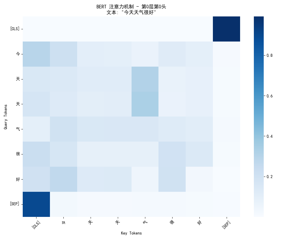
- 坐标轴:
- Y轴(Query):发起关注的token
- X轴(Key):被关注的token
- 颜色深浅:
- 颜色越深(蓝色越深)→ 注意力权重越高
- 颜色越浅 → 注意力权重越低
- 关键观察点:
- 对角线通常较深:每个token都会比较关注自己
- [CLS]行的分布:[CLS]token会相对均匀地关注所有token,因为它要汇总全局信息
- 语义相关的连接:比如"天"和"气"之间可能有较深的连接,因为它们组成"天气"这个词
BERT模型注意力模式分析 ================================================== 输入文本: 今天天气很好适合出门 分词: ['[CLS]', '今', '天', '天', '气', '很', '好', '适', '合', '出', '门', '[SEP]'] 总层数: 12 每层头数: 12 序列长度: 12 第一层第一个头的注意力模式: Query → [最关注的Key Tokens] ---------------------------------------- [CLS] → ['[SEP](0.978)'] 今 → ['[CLS](0.200)', '今(0.145)', '门(0.107)'] 天 → ['气(0.221)', '[CLS](0.105)', '出(0.101)'] 天 → ['气(0.232)', '[CLS](0.121)'] 气 → ['适(0.154)', '出(0.128)', '今(0.117)'] 很 → ['[CLS](0.160)', '很(0.137)', '今(0.117)', '好(0.101)'] 好 → ['今(0.183)', '[CLS](0.139)', '出(0.136)', '很(0.135)'] 适 → ['[CLS](0.219)', '合(0.142)', '气(0.122)'] 合 → ['气(0.197)', '很(0.138)', '门(0.107)', '[CLS](0.105)'] 出 → ['很(0.174)', '今(0.148)', '门(0.134)'] 门 → ['适(0.172)', '[CLS](0.123)', '好(0.115)'] [SEP] → ['[CLS](0.851)'] 第0层的12个注意力头模式: ============================================================ 头 0 的注意力模式: [CLS] → 最关注: [SEP](0.991) 今 → 最关注: [CLS](0.293) 天 → 最关注: 气(0.313) 天 → 最关注: 气(0.330) 气 → 最关注: 今(0.195) 很 → 最关注: [CLS](0.226) 好 → 最关注: 今(0.264) [SEP] → 最关注: [CLS](0.897) 头 1 的注意力模式: [CLS] → 最关注: [SEP](0.930) 今 → 最关注: [CLS](0.425) 天 → 最关注: 今(0.625) 天 → 最关注: 气(0.455) 气 → 最关注: 天(0.628) 很 → 最关注: 好(0.364) 好 → 最关注: 很(0.566) [SEP] → 最关注: [SEP](0.999) 头 2 的注意力模式: [CLS] → 最关注: [CLS](0.890) 今 → 最关注: [CLS](0.760) 天 → 最关注: [CLS](0.767) 天 → 最关注: [CLS](0.665) 气 → 最关注: [CLS](0.633) 很 → 最关注: [CLS](0.466) 好 → 最关注: [CLS](0.508) [SEP] → 最关注: [CLS](0.822) 头 3 的注意力模式: [CLS] → 最关注: 天(0.218) 今 → 最关注: 很(0.366) 天 → 最关注: [SEP](0.270) 天 → 最关注: [SEP](0.277) 气 → 最关注: 好(0.254) 很 → 最关注: 好(0.503) 好 → 最关注: [SEP](0.315) [SEP] → 最关注: 今(0.242)
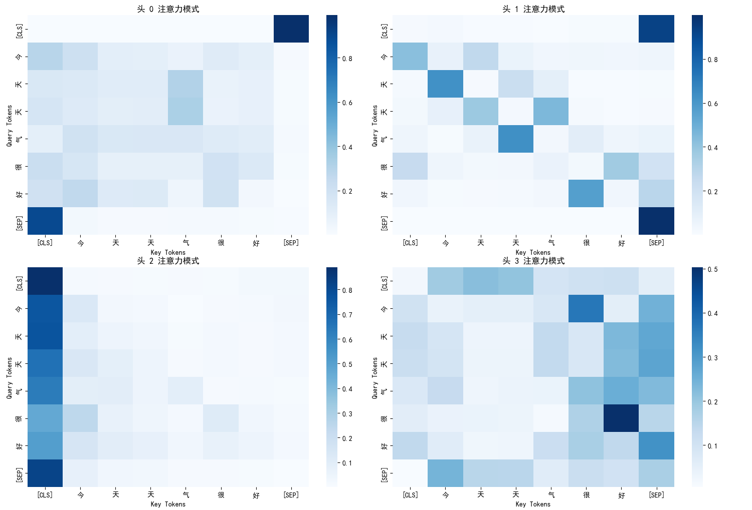
多头注意力的意义:
- BERT有12层,每层有12个注意力头
- 每个头学习不同的注意力模式:
- 头0:可能关注语法关系
- 头1:可能关注语义相关性
- 头2:可能关注位置关系
- 头3:可能关注特定词汇搭配
三、Decoder-only 架构
1. 基础理解
想象一下,我们在玩一个故事接龙的游戏,规则很简单,接着前一个人说的内容,继续叙述后面的情节,直到完成一个完整的故事,在这个游戏里,每个人只能基于前面已经说过的所有内容,来创作下一句话,你无法提前知道后面的人会说什么,也不能修改已经说过的话。
Decoder-only 模型就是这样一位成语接龙高手。它的工作方式是:
- 从起始标记(如 <s>)开始
- 基于当前已有的所有文本,预测下一个最可能的词
- 将新生成的词添加到文本中,重复这个过程
- 直到生成完整的文本或达到结束标记
核心特点:自回归生成,一步接一步。
Decoder-only 模型像一个不知疲倦的创作者,它写小说时,只能从左到右、一个字一个字地写,每写一个新字都要反复阅读前面已经写好的所有内容。
2. 代表模型
GPT 是 Decoder-only 架构最著名的代表,它的名字就揭示了其本质:生成式预训练Transformer。
GPT 的训练目标非常简单直接:预测下一个词。
基础训练:下一个词预测
- 输入:“今天天气很”
- 目标:让模型预测下一个词应该是“好”
- 方法:在海量文本上重复这个练习,让模型学会语言的统计规律
学习成果:
- 学会了语法规则(形容词后面接名词)
- 学会了语义关联(“天气”与“很好”经常一起出现)
- 学会了逻辑推理(如果前面提到“下雨”,后面可能接“带伞”)
- 学会了文体风格(新闻、小说、诗歌的不同写法)
这种简单的训练非常有效,因为要准确预测下一个词,模型必须深刻理解:前文的语法结构、词汇的语义关系、文本的逻辑连贯性、语言的风格特征
3. 核心技术
为了让故事接龙成为可能,Decoder-only 模型采用了一种关键的技术:因果注意力掩码。
如何理解因果注意力掩码:
- 在训练时,模型会看到完整的句子,比如:“今天天气很好”
- 但如果模型在预测“很”字时,能够看到后面的“好”字,这就是作弊!
- 为了避免作弊,必须让模型在预测每个位置时,只能看到当前位置和之前的位置
因果注意力掩码的工作原理:
# 因果注意力模式示意图 输入序列: <s> 今天 天气 很 生成过程: 生成"今天"时 → 只能看到: [<s>] 生成"天气"时 → 只能看到: [<s>, 今天] 生成"很"时 → 只能看到: [<s>, 今天, 天气] 生成"好"时 → 只能看到: [<s>, 今天, 天气, 很]
这就像一个逐步揭开的面纱:
- 开始时,你只能看到第一个词
- 每生成一个新词,面纱就往后移动一点,让你多看到一个词
- 但你永远无法看到面纱后面的未来内容
因果注意力关键特点:
- 1. 单向性: 只能从左到右,不能反向
- 2. 累积性: 每步增加一个新token的访问权限
- 3. 防泄露: 永远不会看到未来的信息
- 4. 自回归: 基于历史预测下一个token
4. 体现优势
擅长所有需要创造性生成的任务
任务类型 | 例子 | 说明 |
|---|---|---|
文本创作 | 写小说、诗歌、新闻稿 | 像作家一样从头创作完整文本 |
对话系统 | 智能客服、聊天机器人 | 基于对话历史生成自然回复 |
内容续写 | 给定开头,完成整篇文章 | 保持风格一致性地扩展内容 |
代码生成 | 根据描述自动写代码 | 理解需求并生成程序代码 |
文本翻译 | 中英文互译 | 将一种语言流畅地转换为另一种 |
5. 局限性
无法利用后文信息
- 在生成过程中,模型看不到未来的内容
- 这有时会导致前后不一致的问题
错误累积
- 如果前面生成错误,后面的内容会基于错误继续生成
- 像传话游戏一样,错误会不断放大
理解深度有限
- 虽然能生成流畅文本,但对深层次语义理解不如Encoder模型
- 有时会一本正经地胡说八道
6. 示例分析
6.1 逐步生成演示
from transformers import AutoModelForCausalLM, AutoTokenizer
import torch
from modelscope import snapshot_download

class DecoderOnlyExample:
    def __init__(self):
        # 使用ModelScope中的GPT系列小模型
        cache_dir = "D:\\modelscope\\hub"
        self.model_name = "Fengshenbang/Wenzhong-GPT2-110M-chinese-v2"
        local_model_path = snapshot_download(self.model_name, cache_dir=cache_dir)
        self.tokenizer = AutoTokenizer.from_pretrained(local_model_path)
        self.model = AutoModelForCausalLM.from_pretrained(local_model_path)

        # 设置padding token
        if self.tokenizer.pad_token is None:
            self.tokenizer.pad_token = self.tokenizer.eos_token

    def generate_text(self, prompt, max_length=100, temperature=0.8):
        """文本生成示例"""
        inputs = self.tokenizer(prompt, return_tensors='pt')

        with torch.no_grad():
            outputs = self.model.generate(
                inputs.input_ids,
                max_length=max_length,
                num_return_sequences=1,
                temperature=temperature,
                do_sample=True,
                pad_token_id=self.tokenizer.eos_token_id,
                no_repeat_ngram_size=3
            )

        generated_text = self.tokenizer.decode(outputs[0], skip_special_tokens=True)
        return generated_text

    def calculate_perplexity(self, text):
        """计算文本困惑度"""
        inputs = self.tokenizer(text, return_tensors='pt')
        with torch.no_grad():
            outputs = self.model(**inputs, labels=inputs.input_ids)
            loss = outputs.loss
            perplexity = torch.exp(loss)
        return perplexity.item()

# 使用示例
decoder_example = DecoderOnlyExample()
prompt = "人工智能的未来发展"
generated_text = decoder_example.generate_text(prompt)
print(f"输入提示: {prompt}")
print(f"生成的文本: {generated_text}")


def simple_causal_attention_demo():
    print("\n" + "="*60)
    """最简单的因果注意力演示"""
    print("因果注意力模式 (Decoder-only)")
    print("=" * 40)

    # 输入序列
    sequence = ["<s>", "今天", "天气", "很"]
    print(f"输入序列: {' '.join(sequence)}")
    print()

    print("注意力模式:")
    print("-" * 25)

    # 为每个位置显示可以关注的位置
    for i in range(len(sequence)):
        current_token = sequence[i]
        # 当前位置可以关注的所有位置(从0到i)
        can_attend = sequence[:i+1]

        print(f"{current_token:4} → {', '.join(can_attend)}")

# 运行演示
simple_causal_attention_demo()

def clear_causal_demo():
    """更清晰的因果注意力演示"""
    print("\n" + "="*60)
    print("Decoder-only 因果注意力")
    print("=" * 35)

    tokens = ["<s>", "今天", "天气", "很", "好"]

    print("规则: 每个token只能关注它自己和前面的所有token")
    print()

    for i in range(len(tokens)):
        current = tokens[i]
        previous = tokens[:i+1]  # 从开始到当前的所有token

        arrow = "→"
        if i == 0:
            arrow = "→ (只能关注自己)"
        elif i == len(tokens) - 1:
            arrow = "→ (可以关注前面所有token)"

        print(f"{current:4} {arrow:20} {', '.join(previous)}")

# 运行清晰版本
clear_causal_demo()

def minimal_demo():
    print("\n" + "="*60)
    """最简化的核心逻辑演示"""
    tokens = ["起始", "今天", "天气", "很", "好"]

    print("因果注意力核心规则:")
    print("每个位置只能看到它和它之前的所有位置")
    print()

    for i in range(len(tokens)):
        can_see = tokens[:i+1]
        print(f"生成 '{tokens[i]}' 时,模型能看到: {can_see}")

# 运行最简版本
minimal_demo()
输出结果:
输入提示: 人工智能的未来发展 生成的文本: 人工智能的未来发展方向-高端人才培养。 春节期间,百度联合国内一些知名人士、研发机构、科砙企业(包 因果注意力模式 (Decoder-only) ============================================================ 输入序列: <s> 今天 天气 很 注意力模式: ------------------------- <s> → <s> 今天 → <s>, 今天 天气 → <s>, 今天, 天气 很 → <s>, 今天, 天气, 很 Decoder-only 因果注意力 ============================================================ 规则: 每个token只能关注它自己和前面的所有token <s> → (只能关注自己) <s> 今天 → <s>, 今天 天气 → <s>, 今天, 天气 很 → <s>, 今天, 天气, 很 好 → (可以关注前面所有token) <s>, 今天, 天气, 很, 好 因果注意力核心规则: ============================================================ 每个位置只能看到它和它之前的所有位置 生成 '起始' 时,模型能看到: ['起始'] 生成 '今天' 时,模型能看到: ['起始', '今天'] 生成 '天气' 时,模型能看到: ['起始', '今天', '天气'] 生成 '很' 时,模型能看到: ['起始', '今天', '天气', '很'] 生成 '好' 时,模型能看到: ['起始', '今天', '天气', '很', '好']
6.2 因果注意力模式分析
import torch
from transformers import AutoModelForCausalLM, AutoTokenizer
import numpy as np
from modelscope import snapshot_download
class CausalAttentionVisualizer:
def __init__(self, model_name="gpt2-chinese-cluecorpussmall"):
cache_dir = "D:\\modelscope\\hub"
self.model_name = "Fengshenbang/Wenzhong-GPT2-110M-chinese-v2"
local_model_path = snapshot_download(self.model_name, cache_dir=cache_dir)
self.tokenizer = AutoTokenizer.from_pretrained(local_model_path)
self.model = AutoModelForCausalLM.from_pretrained(local_model_path, output_attentions=True)
self.model.eval()
if self.tokenizer.pad_token is None:
self.tokenizer.pad_token = self.tokenizer.eos_token
def get_causal_attention_mask(self, seq_len):
"""生成因果注意力掩码"""
# 创建下三角矩阵,1表示允许关注,0表示不允许
mask = torch.tril(torch.ones(seq_len, seq_len))
return mask
def visualize_causal_pattern(self, text):
"""可视化因果注意力模式"""
# 编码文本
inputs = self.tokenizer(text, return_tensors='pt')
seq_len = inputs['input_ids'].shape[1]
print("因果注意力模式分析")
print("=" * 40)
print(f"序列长度: {seq_len}")
print(f"输入序列: {text}")
print("\n注意力模式:")
print("-" * 30)
# 生成因果注意力掩码
causal_mask = self.get_causal_attention_mask(seq_len)
# 输出注意力模式
for i in range(seq_len):
# 获取当前位置可以关注的token索引
allowed_indices = torch.where(causal_mask[i] == 1)[0].tolist()
if i == 0:
# 第一个token只能关注自己
print(f"位置 {i} → [位置 {i}]")
else:
# 其他位置可以关注从0到当前位置的所有token
positions = [f"位置 {j}" for j in allowed_indices]
print(f"位置 {i} → {positions}")
return causal_mask
# 使用示例
visualizer = CausalAttentionVisualizer()
text = "今天天气很"
causal_mask = visualizer.visualize_causal_pattern(text)
def analyze_causal_attention_detailed():
"""详细分析因果注意力模式"""
visualizer = CausalAttentionVisualizer()
text = "今天天气很好适合出门"
inputs = visualizer.tokenizer(text, return_tensors='pt')
seq_len = inputs['input_ids'].shape[1]
print("Decoder-only 因果注意力机制")
print("=" * 50)
print(f"输入序列长度: {seq_len}")
print("\n完整的注意力模式矩阵:")
print("-" * 40)
# 生成因果注意力掩码
causal_mask = visualizer.get_causal_attention_mask(seq_len)
# 输出矩阵形式的注意力模式
print(" ", end="")
for j in range(seq_len):
print(f"{j:2} ", end="")
print()
for i in range(seq_len):
print(f"{i:2} ", end="")
for j in range(seq_len):
if causal_mask[i, j] == 1:
print(" ● ", end="")
else:
print(" · ", end="")
print(f" 位置 {i} 可以关注: {[k for k in range(seq_len) if causal_mask[i, k] == 1]}")
print("\n其中: ● = 允许关注, · = 禁止关注")
# 运行详细分析
analyze_causal_attention_detailed()
def verify_model_attention():
"""验证实际模型的因果注意力"""
visualizer = CausalAttentionVisualizer()
text = "今天天气很"
inputs = visualizer.tokenizer(text, return_tensors='pt')
with torch.no_grad():
outputs = visualizer.model(**inputs, output_attentions=True)
attentions = outputs.attentions # 所有层的注意力
seq_len = inputs['input_ids'].shape[1]
print("实际模型因果注意力验证")
print("=" * 40)
print(f"模型层数: {len(attentions)}")
print(f"每层头数: {attentions[0].shape[1]}")
print(f"序列长度: {seq_len}")
# 检查第一层第一个头的注意力
first_head_attention = attentions[0][0, 0] # [seq_len, seq_len]
print("\n第一层第一个头注意力模式:")
print("位置 → [可以关注的位置] (注意力权重>0.01)")
print("-" * 50)
for i in range(seq_len):
# 找出有显著注意力权重的位置
significant_positions = []
for j in range(seq_len):
if first_head_attention[i, j] > 0.01:
significant_positions.append(j)
print(f"位置 {i} → 位置 {significant_positions}")
# 验证模型注意力
verify_model_attention()
import matplotlib.pyplot as plt
# 设置中文字体
plt.rcParams['font.sans-serif'] = ['SimHei']
plt.rcParams['axes.unicode_minus'] = False
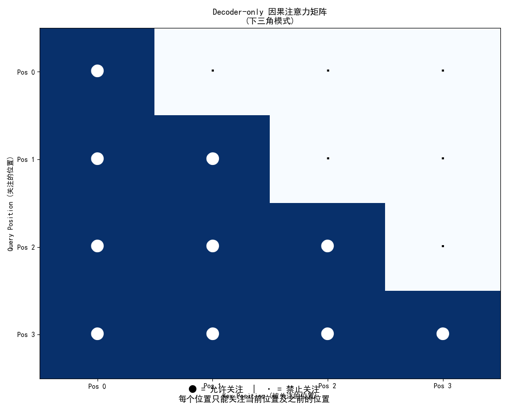
def plot_causal_attention_matrix(seq_len=6):
"""绘制因果注意力矩阵图"""
# 创建因果注意力掩码
causal_mask = torch.tril(torch.ones(seq_len, seq_len))
plt.figure(figsize=(10, 8))
plt.imshow(causal_mask, cmap='Blues', aspect='auto')
# 添加网格和标签
for i in range(seq_len):
for j in range(seq_len):
color = 'white' if causal_mask[i, j] > 0.5 else 'black'
plt.text(j, i, '●' if causal_mask[i, j] > 0.5 else '·',
ha='center', va='center', color=color, fontsize=20)
plt.xlabel('Key Position (被关注的位置)')
plt.ylabel('Query Position (关注的位置)')
plt.title('Decoder-only 因果注意力矩阵\n(下三角模式)')
plt.xticks(range(seq_len), [f'Pos {i}' for i in range(seq_len)])
plt.yticks(range(seq_len), [f'Pos {i}' for i in range(seq_len)])
plt.grid(False)
# 添加解释
plt.figtext(0.5, 0.01,
'● = 允许关注 | · = 禁止关注\n每个位置只能关注当前位置及之前的位置',
ha='center', fontsize=12, style='italic')
plt.tight_layout()
plt.show()
# 绘制注意力矩阵
plot_causal_attention_matrix(4)因果注意力模式分析 ======================================== 序列长度: 8 输入序列: 今天天气很 注意力模式: ------------------------------ 位置 0 → [位置 0] 位置 1 → ['位置 0', '位置 1'] 位置 2 → ['位置 0', '位置 1', '位置 2'] 位置 3 → ['位置 0', '位置 1', '位置 2', '位置 3'] 位置 4 → ['位置 0', '位置 1', '位置 2', '位置 3', '位置 4'] 位置 5 → ['位置 0', '位置 1', '位置 2', '位置 3', '位置 4', '位置 5'] 位置 6 → ['位置 0', '位置 1', '位置 2', '位置 3', '位置 4', '位置 5', '位置 6'] 位置 7 → ['位置 0', '位置 1', '位置 2', '位置 3', '位置 4', '位置 5', '位置 6', '位置 7']
Decoder-only 因果注意力机制 ================================================== 输入序列长度: 18 完整的注意力模式矩阵: ---------------------------------------- 0 1 2 3 4 5 6 7 8 9 10 11 12 13 14 15 16 17 0 ● · · · · · · · · · · · · · · · · · 位置 0 可以关注: [0] 1 ● ● · · · · · · · · · · · · · · · · 位置 1 可以关注: [0, 1] 2 ● ● ● · · · · · · · · · · · · · · · 位置 2 可以关注: [0, 1, 2] 3 ● ● ● ● · · · · · · · · · · · · · · 位置 3 可以关注: [0, 1, 2, 3] 4 ● ● ● ● ● · · · · · · · · · · · · · 位置 4 可以关注: [0, 1, 2, 3, 4] 5 ● ● ● ● ● ● · · · · · · · · · · · · 位置 5 可以关注: [0, 1, 2, 3, 4, 5] 6 ● ● ● ● ● ● ● · · · · · · · · · · · 位置 6 可以关注: [0, 1, 2, 3, 4, 5, 6] 7 ● ● ● ● ● ● ● ● · · · · · · · · · · 位置 7 可以关注: [0, 1, 2, 3, 4, 5, 6, 7] 8 ● ● ● ● ● ● ● ● ● · · · · · · · · · 位置 8 可以关注: [0, 1, 2, 3, 4, 5, 6, 7, 8] 9 ● ● ● ● ● ● ● ● ● ● · · · · · · · · 位置 9 可以关注: [0, 1, 2, 3, 4, 5, 6, 7, 8, 9] 10 ● ● ● ● ● ● ● ● ● ● ● · · · · · · · 位置 10 可以关注: [0, 1, 2, 3, 4, 5, 6, 7, 8, 9, 10] 11 ● ● ● ● ● ● ● ● ● ● ● ● · · · · · · 位置 11 可以关注: [0, 1, 2, 3, 4, 5, 6, 7, 8, 9, 10, 11] 12 ● ● ● ● ● ● ● ● ● ● ● ● ● · · · · · 位置 12 可以关注: [0, 1, 2, 3, 4, 5, 6, 7, 8, 9, 10, 11, 12] 13 ● ● ● ● ● ● ● ● ● ● ● ● ● ● · · · · 位置 13 可以关注: [0, 1, 2, 3, 4, 5, 6, 7, 8, 9, 10, 11, 12, 13] 14 ● ● ● ● ● ● ● ● ● ● ● ● ● ● ● · · · 位置 14 可以关注: [0, 1, 2, 3, 4, 5, 6, 7, 8, 9, 10, 11, 12, 13, 14] 15 ● ● ● ● ● ● ● ● ● ● ● ● ● ● ● ● · · 位置 15 可以关注: [0, 1, 2, 3, 4, 5, 6, 7, 8, 9, 10, 11, 12, 13, 14, 15] 16 ● ● ● ● ● ● ● ● ● ● ● ● ● ● ● ● ● · 位置 16 可以关注: [0, 1, 2, 3, 4, 5, 6, 7, 8, 9, 10, 11, 12, 13, 14, 15, 16] 17 ● ● ● ● ● ● ● ● ● ● ● ● ● ● ● ● ● ● 位置 17 可以关注: [0, 1, 2, 3, 4, 5, 6, 7, 8, 9, 10, 11, 12, 13, 14, 15, 16, 17] 其中: ● = 允许关注, · = 禁止关注
7. 图解说明
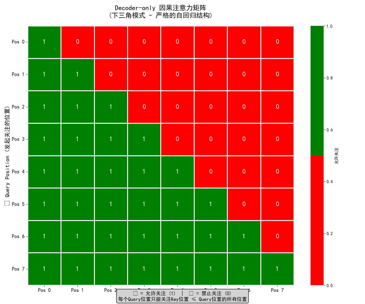
因果注意力模式: -------------------------------------------------- 📍 位置 0 (起始位置) └── 只能关注: [位置 0] ← 自身 └── 意义: 序列开始,无历史信息 📍 位置 1 └── 可以关注: 位置 [0, 1] └── 新增关注: 位置 1 ← 当前生成的位置 └── 历史信息: 1 个之前的位置 📍 位置 2 └── 可以关注: 位置 [0, 1, 2] └── 新增关注: 位置 2 ← 当前生成的位置 └── 历史信息: 2 个之前的位置 📍 位置 3 └── 可以关注: 位置 [0, 1, 2, 3] └── 新增关注: 位置 3 ← 当前生成的位置 └── 历史信息: 3 个之前的位置 📍 位置 4 └── 可以关注: 位置 [0, 1, 2, 3, 4] └── 新增关注: 位置 4 ← 当前生成的位置 └── 历史信息: 4 个之前的位置 📍 位置 5 └── 可以关注: 位置 [0, 1, 2, 3, 4, 5] └── 新增关注: 位置 5 ← 当前生成的位置 └── 历史信息: 5 个之前的位置 📍 位置 6 └── 可以关注: 位置 [0, 1, 2, 3, 4, 5, 6] └── 新增关注: 位置 6 ← 当前生成的位置 └── 历史信息: 6 个之前的位置 📍 位置 7 └── 可以关注: 位置 [0, 1, 2, 3, 4, 5, 6, 7] └── 新增关注: 位置 7 ← 当前生成的位置 └── 历史信息: 7 个之前的位置
四、总结对比
特性 | Decoder-only (如 GPT) | Encoder-only (如 BERT) |
|---|---|---|
核心能力 | 连续生成 | 深度理解 |
工作方式 | 单向自回归,逐个生成 | 双向,同时处理全部输入 |
注意力机制 | 因果注意力(掩码) | 全连接注意力 |
训练目标 | 预测下一个词 | 完形填空、句间关系 |
典型任务 | 写作、对话、翻译、代码生成 | 分类、标注、问答、情感分析 |
比喻 | 故事创作家、脱口秀演员 | 阅读理解大师、分析师 |
选择的决策:
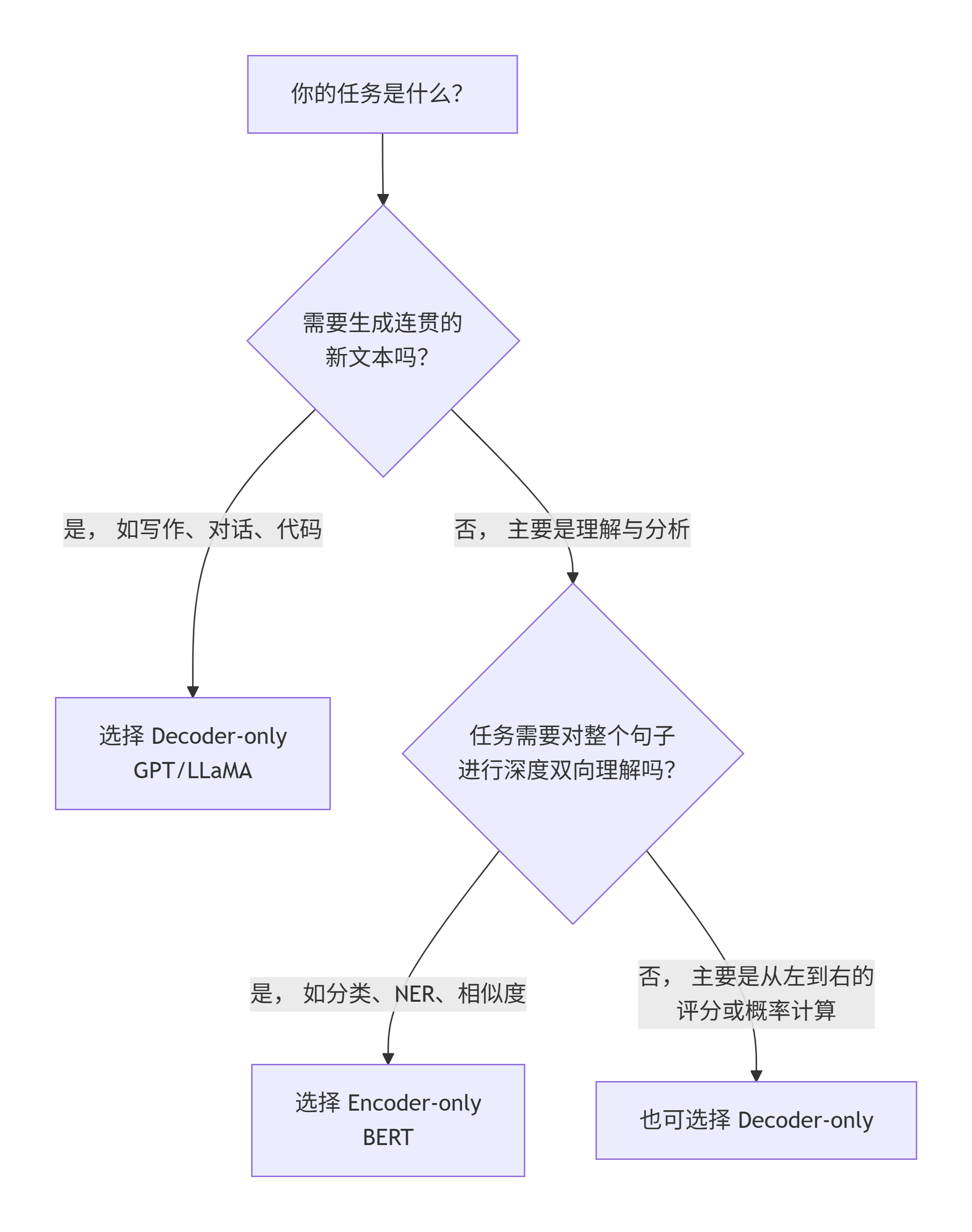
- 当我们需要对一段文本进行深度剖析、分类、提取信息或比较时,Encoder-only (BERT) 是更专业、更高效的工具。
- 当我们需要模型创作内容、进行对话、根据指令完成任务或续写故事时,Decoder-only (GPT) 是唯一的选择。
综合来说,Encoder-only与Decoder-only架构代表了两种截然不同的设计哲学,Encoder-only如BERT,凭借双向注意力机制成为“理解大师”,擅长文本分类、情感分析等深度语义理解任务,为企业提供精准的文本分析能力。而Decoder-only如GPT系列,通过因果注意力掩码实现自回归生成,化身为创作高手,在文本生成、对话系统和代码创作等场景表现卓越。
原创声明:本文系作者授权腾讯云开发者社区发表,未经许可,不得转载。
如有侵权,请联系 cloudcommunity@tencent.com 删除。
原创声明:本文系作者授权腾讯云开发者社区发表,未经许可,不得转载。
如有侵权,请联系 cloudcommunity@tencent.com 删除。
评论
登录后参与评论
推荐阅读
目录
腾讯云开发者

Copyright © 2013 - 2026 Tencent Cloud. All Rights Reserved. 腾讯云 版权所有
深圳市腾讯计算机系统有限公司 ICP备案/许可证号:粤B2-20090059 ![]() 粤公网安备44030502008569号
粤公网安备44030502008569号
腾讯云计算(北京)有限责任公司 京ICP证150476号 | 京ICP备11018762号