GRSA富集：可视化天花板你值得拥有

生信菜鸟团

发布于 2025-01-07 14:19:15

6600

文章被收录于专栏：生信菜鸟团生信菜鸟团

常用的功能富集分析方法，根据其所采用的统计方法大致可分为三类：

（i）过度表达分析（ORA）
（ii）功能类别评分（FCS）
（iii）基于通路拓扑结构（PT）

最近我们介绍了好几种功能富集分析的包，这次又来了一个，个人比较喜欢的，里面可以绘制各种高分文章中出现的富集结果精美展示图，来看看~

文献信息：

Chen Peng, Qiong Chen, Shangjin Tan, Xiaotao Shen, Chao Jiang, Generalized reporter score-based enrichment analysis for omics data, Briefings in Bioinformatics, Volume 25, Issue 3, May 2024, bbae116, https://doi.org/10.1093/bib/bbae116

ReporterScore工具地址：https://cran.r-project.org/web/packages/ReporterScore

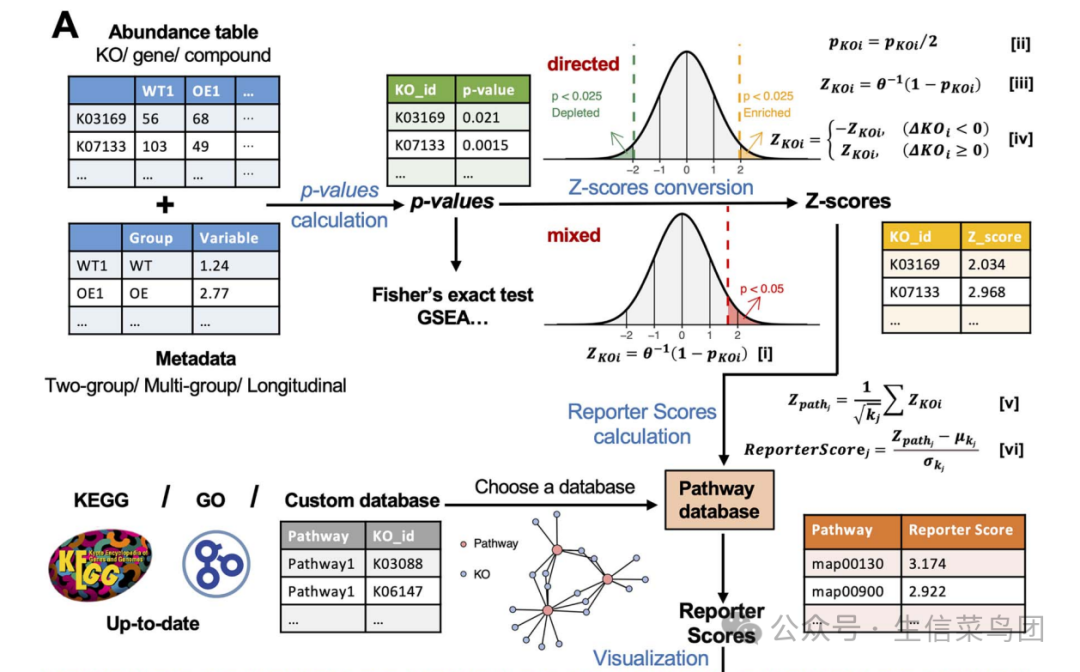
GRSA算法

(1) Calculating the P-values 计算pvalue

pvalue计算方法有以下这些：t检验，wilcoxon秩和检验，ANOVA检验等，更多见supplementary Table S1

(2) pvalue转换为z-score

(3) 对通路进行打分

(4) 最后进行可视化

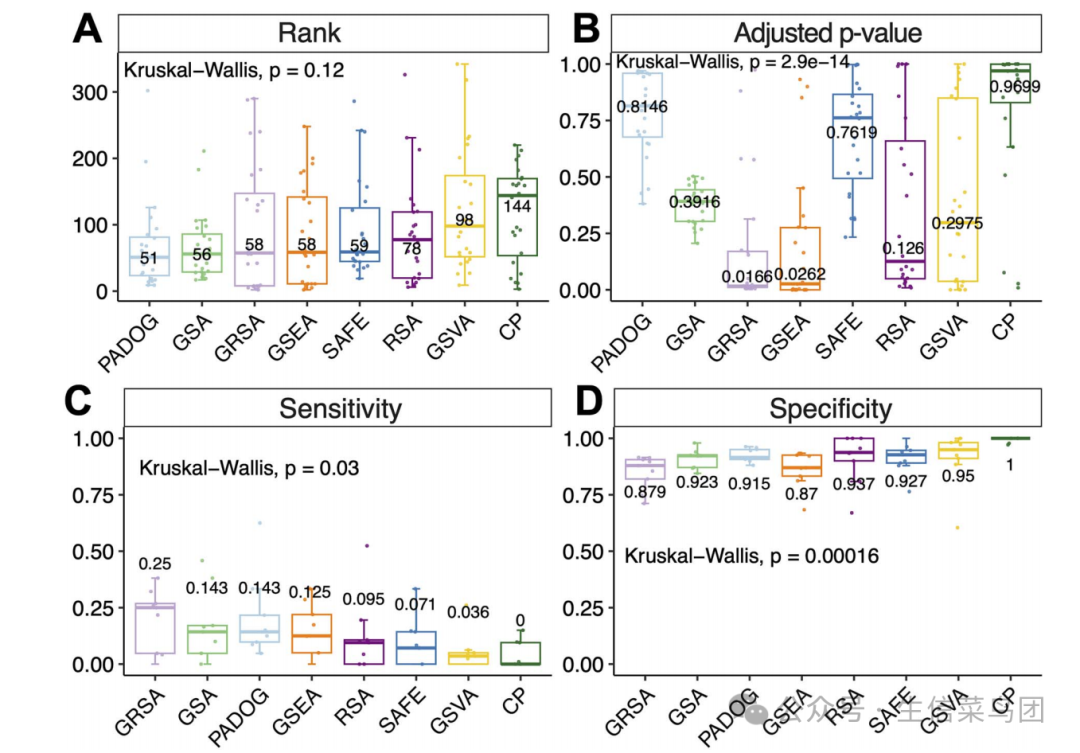
GSRA算法性能比较

使用相同的通路数据库（KEGG v109.0）评估GRSA与其他流行的富集分析方法的性能：GRSA在无阈值的FCS方法中表现相当好，优于传统的ORA方法。

案例使用

1、软件安装：

# 安装cran上的包
options(BioC_mirror="https://mirrors.westlake.edu.cn/bioconductor")
options("repos"=c(CRAN="https://mirrors.westlake.edu.cn/CRAN/"))

install.packages("ReporterScore")

# 或者github上
# install.packages("devtools")
devtools::install_github("Asa12138/pcutils")
devtools::install_github("Asa12138/ReporterScore")

# 检测安装成功与否并加载
library(ReporterScore)

2、输入数据要求

数据为feature丰度数据如基因表达矩阵和样本metadata信息

对于转录组学、单细胞RNA测序（scRNA-seq）以及相关的基于基因的组学数据：可以使用完整的基因丰度表。
对于宏基因组学和宏转录组学数据：可以使用KO（KEGG Orthology）丰度表，该表通过使用Blast、Diamond或KEGG官方映射软件将读取序列或contigs与KEGG或EggNOG数据库进行blast来生成。
对于代谢组学数据：可以使用注释过的化合物丰度表，但需要对化合物ID进行标准化（例如，将化合物ID转换为KEGG数据库中的C编号）。
输入的表格值：可以是 read counts or normalized values (e.g., TPM, FPKM, RPKM, or relative abundance, corresponds to suitable statistical test method).
注意：输入的特征丰度表格不要过滤，以保留所有的背景id信息

metadata：为一个数据框，行为样本，列为样本的表型信息，可以是分类变量也可以是连续变量

注意：metadata的行名与丰度矩阵的列名必须一一对应

下面是一个 KO abundance table 数据示例：

# 示例数据
data("KO_abundance_test")

# 查看前6行
head(KO_abundance[, 1:6])
#>                WT1         WT2         WT3         WT4         WT5         WT6
#> K03169 0.002653545 0.005096380 0.002033923 0.000722349 0.003468322 0.001483028
#> K07133 0.000308237 0.000280458 0.000596527 0.000859854 0.000308719 0.000878098
#> K03088 0.002147068 0.002030742 0.003797459 0.004161979 0.002076596 0.003091182
#> K03530 0.003788366 0.000239298 0.000445817 0.000557271 0.000222969 0.000529624
#> K06147 0.000785654 0.001213630 0.001312569 0.001662740 0.002387006 0.001725797
#> K05349 0.001816325 0.002813642 0.003274701 0.001089906 0.002371921 0.001795214

head(metadata)
#>     Group Group2
#> WT1    WT     G3
#> WT2    WT     G3
#> WT3    WT     G3
#> WT4    WT     G3
#> WT5    WT     G3
#> WT6    WT     G1

# 查看行列名对应
all(rownames(metadata) %in% colnames(KO_abundance))
## TRUE

intersect(rownames(metadata), colnames(KO_abundance))>0
## TRUE

3、通路数据库

ReporterScore包内置了KEGG通路、模块、基因、化合物和GO（Gene Ontology，基因本体论）数据库，并且还允许使用自定义数据库，这样能够与来自多种组学数据的特征丰度表兼容。

# 1. KEGG pathway-KO and module-KO databases
KOlist <- load_KOlist()
head(KOlist$pathway)

# 2. KEGG pathway-compound and module-compound databases
CPDlist <- load_CPDlist()
head(CPDlist$pathway)

# 3. human (hsa) pathway-ko/gene/compound databases
hsa_pathway_gene <- custom_modulelist_from_org(
  org = "hsa",
  feature = c("ko", "gene", "compound")[2]
)
head(hsa_pathway_gene)

# 4. GO-gene database
GOlist <- load_GOlist()
head(GOlist$BP)

# 5. 还可以使用下面的函数自定于通路数据库
?custom_modulelist()

4、运行GRSA

使用 GRSA 函数一步运行得到富集结果，其重要参数如下：

mode：可选 “mixed” 或 “directed”，directed为组间比较分析模式，可以知道通路在哪个组别中显著富集或减少
method：统计学方法，计算每条通路的pvalue，可选 t.test，wilcox.test、anova、kruskal.test等
type：选择内置数据库，pathway 或 module 为 KEGG database；‘CC’, ‘MF’, ‘BP’, ‘ALL’为GO数据库
modulelist：自定义数据库
feature：特征属性，可以为“ko”, “gene”, “compound”.

接下来，以比较两个组别‘WT-OE’（野生型-过表达）为例子，使用“定向”模式，探索在OE组中哪些通路是富集或减少的。

cat("Comparison: ", levels(factor(metadata$Group)), "\n")
#> Comparison:  WT OE

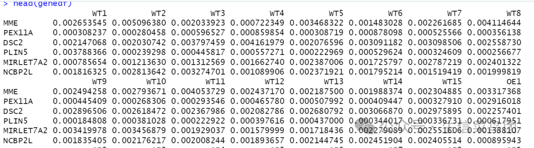
data("genedf")
head(genedf)

数据为一个基因水平的表达矩阵：

GRSA分析：

# Method 1: Set the `feature` and `type`!
reporter_res_gene <- GRSA(genedf, 
                          "Group", 
                          metadata,
                          mode = "directed",
                          method = "wilcox.test", 
                          perm = 999,
                          type = "hsa", 
                          feature = "gene")
                          
## 探索一下结果格式
class(reporter_res_gene)
head(reporter_res_gene)
str(reporter_res_gene)

# view data.frame in Rstudio
View(reporter_res$reporter_s)

# export result as .csv and check using Excel:
export_report_table(reporter_res, dir_name = "./")

生成的结果是一个list对象：

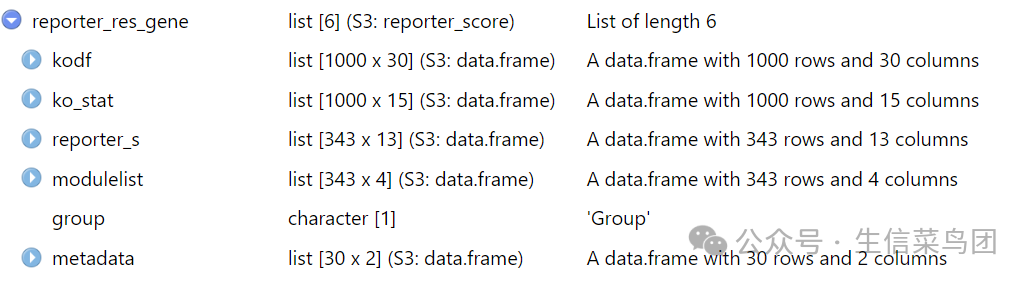
kodf：输入的 KO_abundance 表格
ko_stat：ko 统计结果，包括pvalue和z.score
reporter_s：每条通路的reporter打分
modulelist：自定义的 modulelist 或者 KOlist数据框
group：样本分组
metadata：样本表型metadata数据框

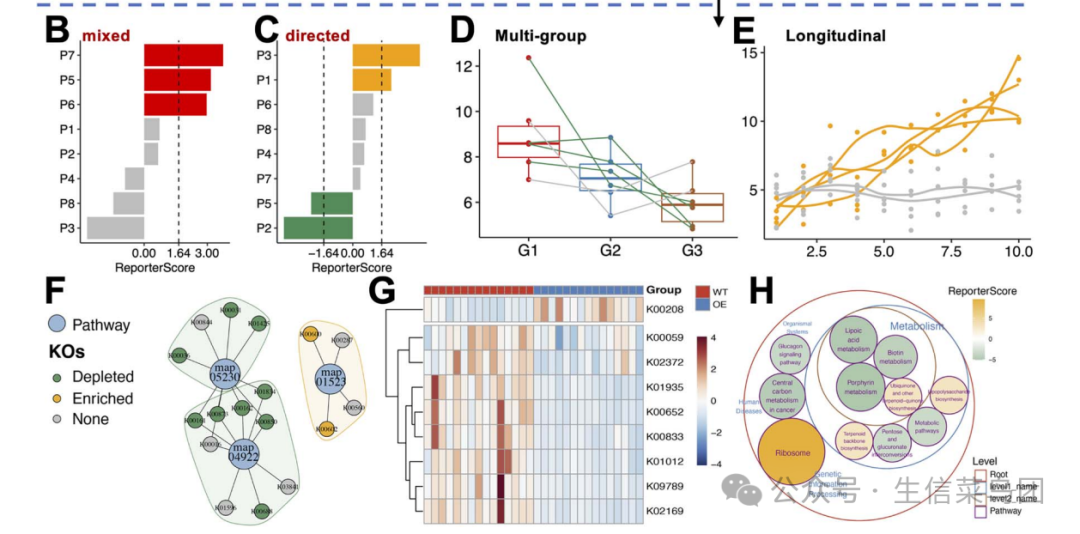
5、结果可视化

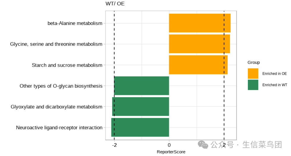
得到 reporter 打分后，可以绘制最显著的富集到的 pathways。

# Use `modify_description` to remove the suffix of pathway description
reporter_res_gene2 <- modify_description(reporter_res_gene, pattern = " - Homo sapiens (human)")
p2 <- plot_report_bar(reporter_res_gene2, rs_threshold = 2)
p2

结果如下：

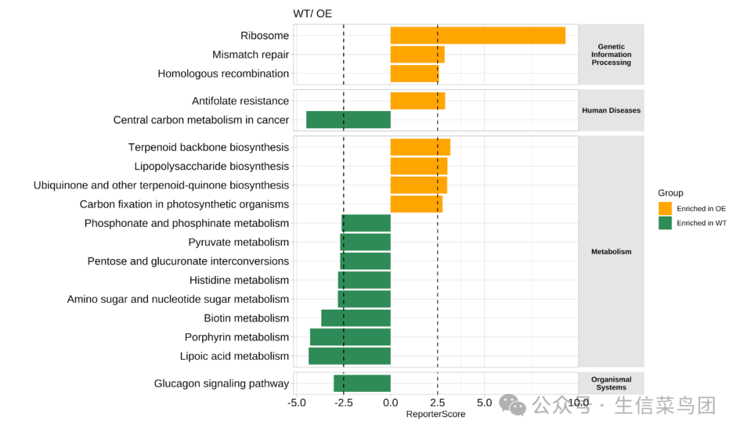
还可以展示KEGG通路的分类：

# View(reporter_res$reporter_s)
plot_report_bar(reporter_res, rs_threshold = c(-2.5, 2.5), facet_level = TRUE)

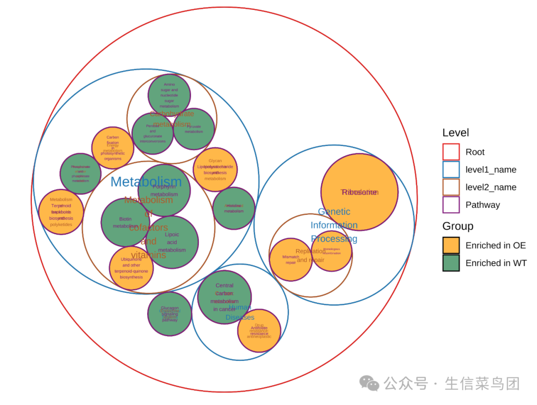
还可以使用圈图风格，这个在代谢和微生物组学中出现的比较多：

plot_report_circle_packing(reporter_res, rs_threshold = c(-2.5, 2.5))

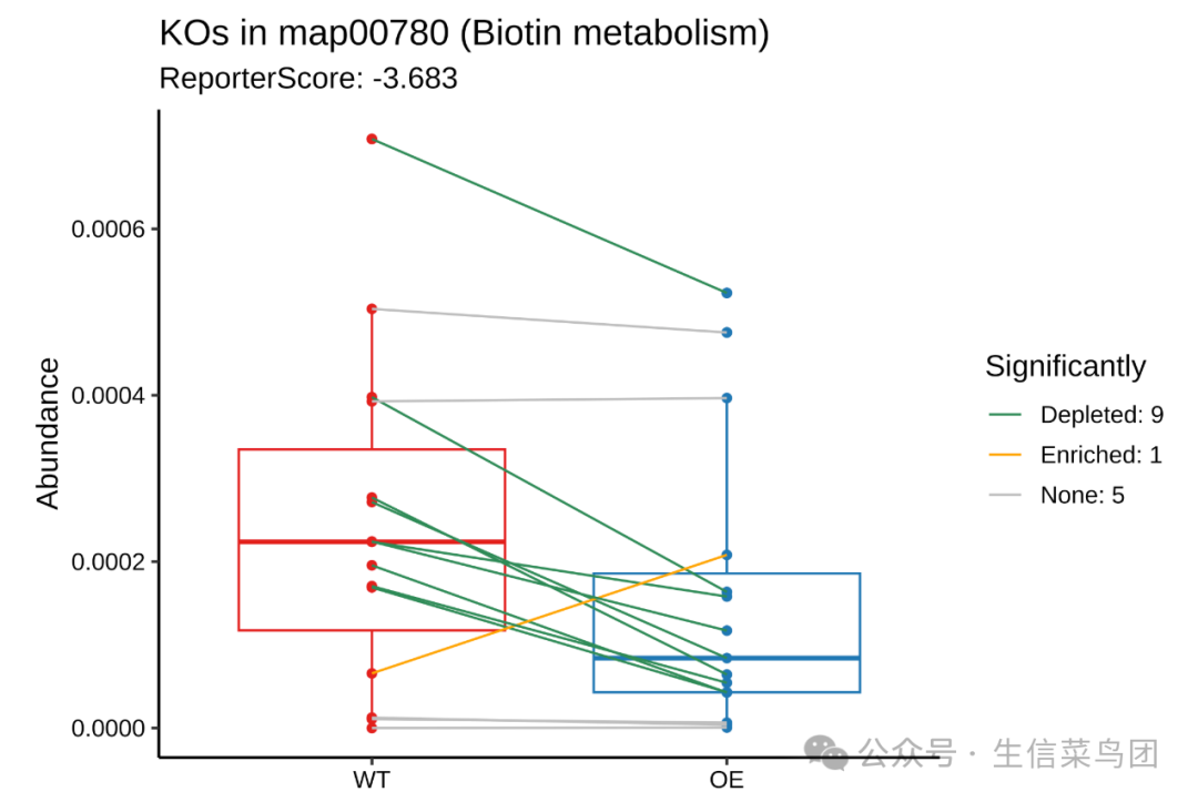
绘制某一条通路的箱线图：map00780

plot_KOs_in_pathway(reporter_res, map_id = "map00780")

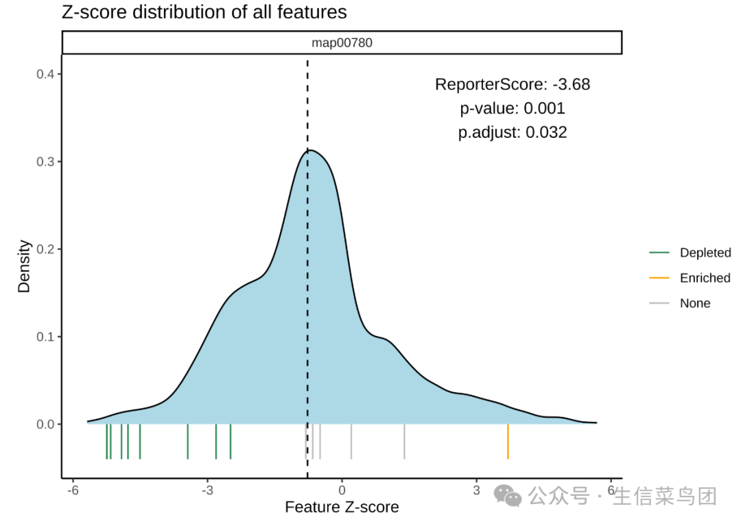
Z-scores分布：

plot_KOs_distribution(reporter_res, map_id = "map00780")

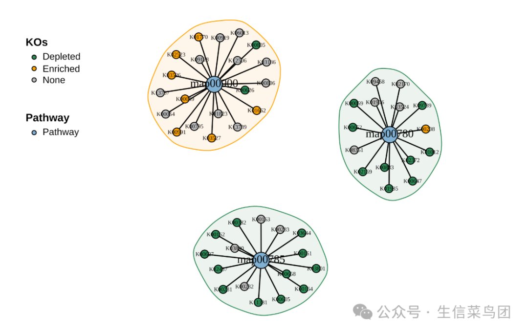
不同通路的网络图：

plot_KOs_network(reporter_res,
  map_id = c("map00780", "map00785", "map00900"),
  main = "", mark_module = TRUE
)

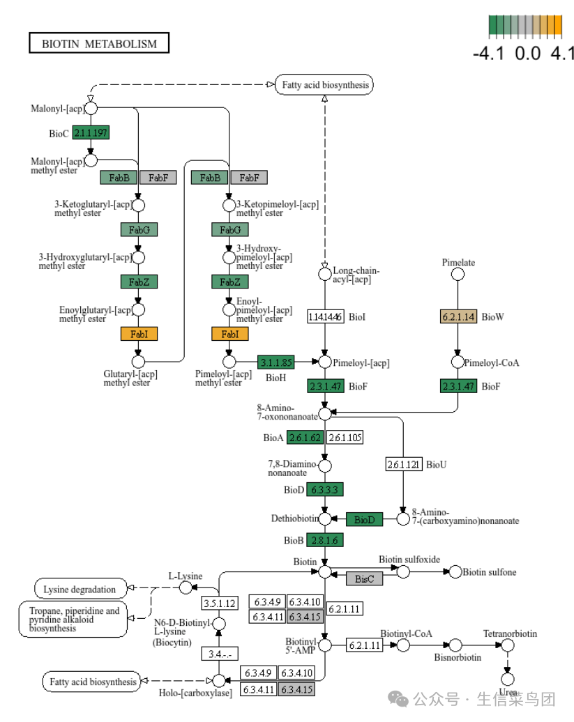
KEGG pathway map图：

plot_KEGG_map(reporter_res, map_id = "map00780", color_var = "Z_score")

其他

还有多分组比较以及其他更多好看的可视化结果，去看看吧~

前面介绍过的其他功能富集分析：

新秀mulea包能取代y叔的clusterProfiler包生物学功能富集分析吗？

本文参与腾讯云自媒体同步曝光计划，分享自微信公众号。

原始发表：2025-01-05，如有侵权请联系 cloudcommunity@tencent.com 删除

数据库

本文分享自生信菜鸟团微信公众号，前往查看

如有侵权，请联系 cloudcommunity@tencent.com 删除。

本文参与腾讯云自媒体同步曝光计划，欢迎热爱写作的你一起参与！

登录后参与评论

0 条评论

热度