🤩 shapviz | 如何利用SHAP解释Xgboost模型！?~

生信漫卷

发布于 2024-02-01 15:34:21

5.4K0

文章被收录于专栏：R语言及实用科研软件R语言及实用科研软件

1写在前面

今天讲一下机器学习的经典方法，SHAP（Shapley Additive exPlanations）。🤒

SHAP使用来自博弈论及其相关扩展的经典Shapley value将最佳信用分配与局部解释联系起来，是一种基于游戏理论上最优的Shapley value来解释个体预测的方法。😂

从博弈论的角度，把data中的每一个特征变量当成一个玩家，用这个data去训练模型得到预测的结果，可以看成众多玩家合作完成一个项目的收益。🙃

Shapley value通过考虑各个玩家做出的贡献，来公平的分配合作的收益。🤓

SHAP值可以可靠地解释树模型。🌲

2用到的包

rm(list = ls())
#devtools::install_github("ModelOriented/shapviz")
library(shapviz)
library(xgboost)
library(tidyverse)
library(patchwork)

3示例数据

x <- c("carat", "cut", "color", "clarity")

data("diamonds")

4建模

这里我们利用一下xgboost建模。😘

dtrain <- xgb.DMatrix(data.matrix(diamonds[x]), label = diamonds$price, nthread = 1)

fit <- xgb.train(params = list(learning_rate = 0.1, nthread = 1), data = dtrain, nrounds = 65)

fit

5shap分析并简单可视化

dia_2000 <- diamonds[sample(nrow(diamonds), 2000), x]

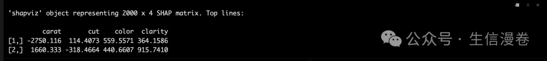
shp <- shapviz(fit, X_pred = data.matrix(dia_2000), X = dia_2000)

shp

经典barplot。😘

sv_importance(shp, show_numbers = T)

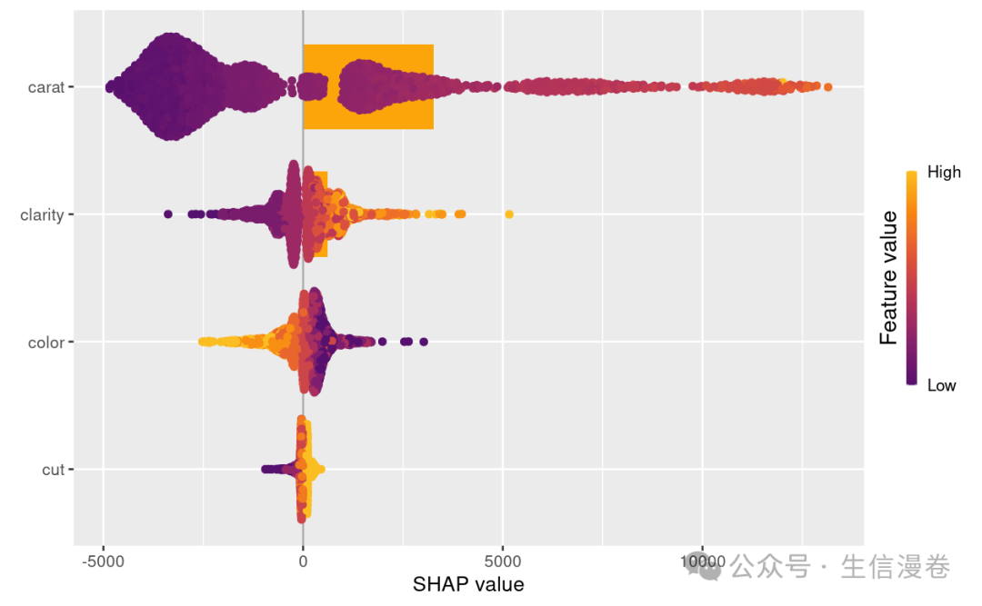
换个姿势，再来一次！~😘

这里我们把蜂群图也加进来，点沿每个特征行堆积以显示密度。🤓

颜色用于显示特征的原始值。🥳

sv_importance(shp, kind = "both")  # "bar", "beeswarm", "both", "no"

6依赖图

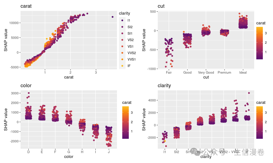
依赖图展示的是一个或两个特征对机器学习模型的预测结果的边际效应，可以显示目标和特征之间的关系。😘

展示的是一个特征的值与该特征的SHAP值。😜

依赖图的一个重要假设是第一个特征与第二个特征不相关。⭐️

有时候特征间存在交互效应，这个时候可以通过加入第二个特征来显示，这里是点的颜色。🫠

sv_dependence(shp, v = x)

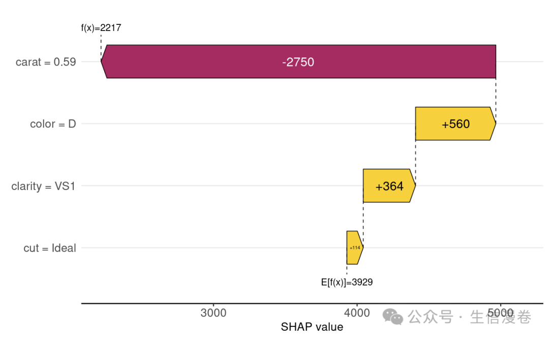
7模型预测的可解释

瀑布图。🙊

sv_waterfall(shp, row_id = 1) +
  theme(axis.text = element_text(size = 11))

Force plot，这里看下第一个。😘

sv_force(shp, row_id = 1)

你也可以选择特征的属性，比如这里选beautiful color D diamonds。😏

sv_waterfall(shp, shp$X$color == "D") +
  theme(axis.text = element_text(size = 11))

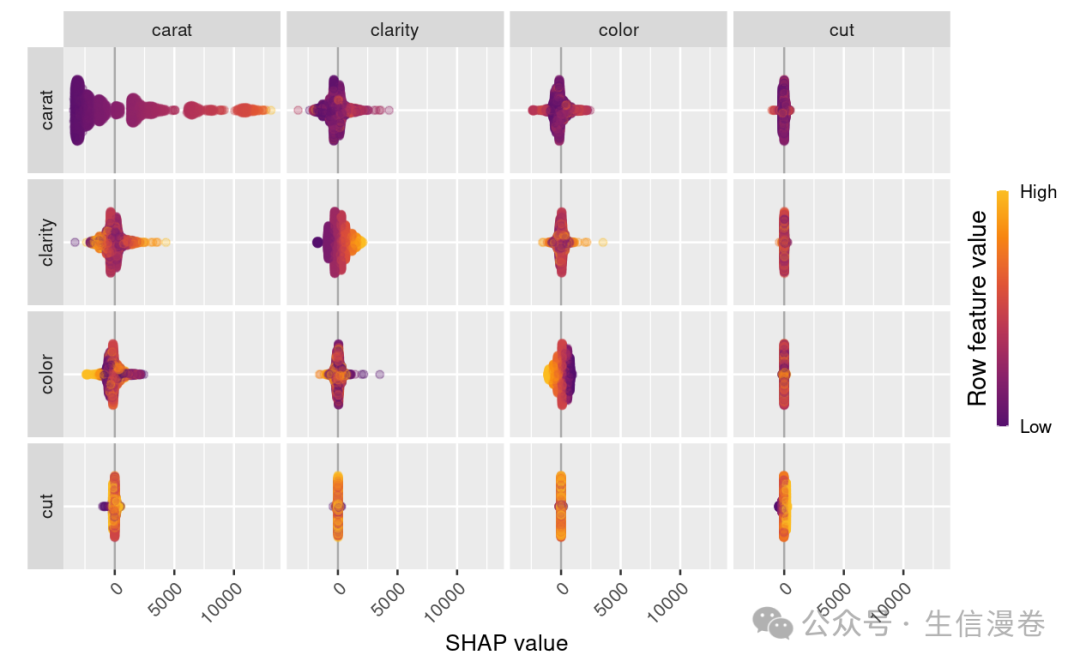
8SHAP Interactions

interaction value是SHAP值更高阶的一种玩法，完美展示交互效应。😘

首先计算一下。🤓

shp_i <- shapviz(fit, X_pred = data.matrix(dia_2000[x]), X = dia_2000, interactions = T)

shp_i

依赖图展示。🐡

sv_dependence(shp_i, v = "carat", color_var = x, interactions = T)

一目了然，perfect！~🎱

sv_interaction(shp_i) +
  theme(axis.text.x = element_text(angle = 45, vjust = 1, hjust = 1))

本文参与腾讯云自媒体同步曝光计划，分享自微信公众号。

原始发表：2024-01-29，如有侵权请联系 cloudcommunity@tencent.com 删除

xgboost

本文分享自生信漫卷微信公众号，前往查看

如有侵权，请联系 cloudcommunity@tencent.com 删除。

本文参与腾讯云自媒体同步曝光计划，欢迎热爱写作的你一起参与！

登录后参与评论

0 条评论

热度