分割环，即R中的非满对象(在EBIimage或其他方面)

Question

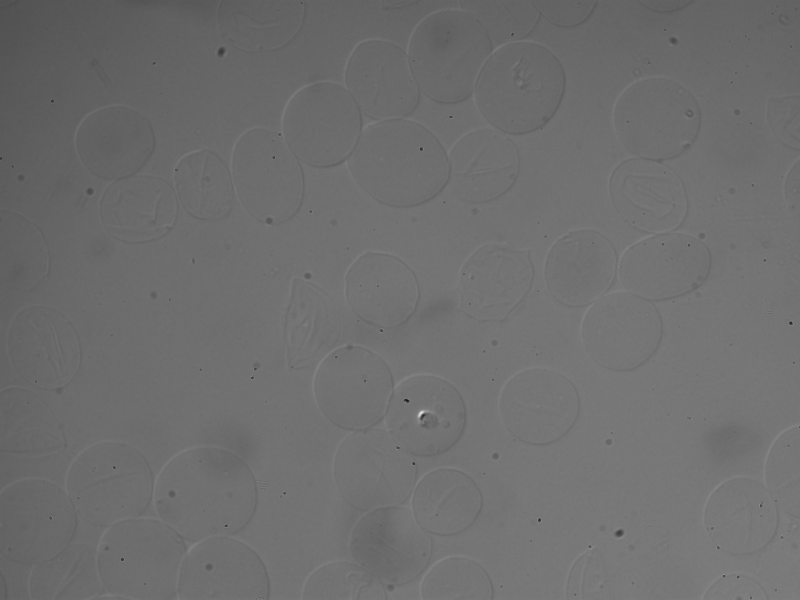
我依靠边缘检测(相对于颜色检测)从血细胞中提取特征。原始图像如下：

​

​

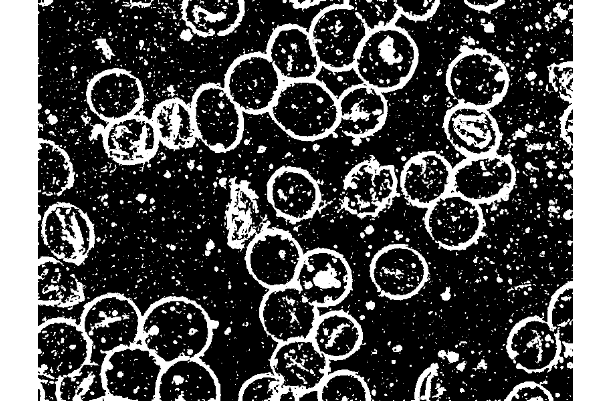
我正在使用R EBImage包运行sobel +低通滤波器来实现这样的功能：

​

​

library(EBImage)
library(data.table)
img <- readImage("6hr-007-DIC.tif")

#plot(img)


#print(img, short = T)

# 1. define filter for edge detection
hfilt <- matrix(c(1, 2, 1, 0, 0, 0, -1, -2, -1), nrow = 3) # sobel

# rotate horizontal filter to obtain vertical filter
vfilt <- t(hfilt)

# get horizontal and vertical edges
imgH <- filter2(img, hfilt, boundary="replicate")
imgV <- filter2(img, vfilt, boundary="replicate")

# combine edge pixel data to get overall edge data
hdata <- imageData(imgH)
vdata <- imageData(imgV)
edata <- sqrt(hdata^2 + vdata^2)

# transform edge data to image
imgE <- Image(edata)
#print(display(combine(img, imgH, imgV, imgE), method = "raster", all = T))

display(imgE, method = "raster", all = T)


# 2. Enhance edges with low pass filter

hfilt <- matrix(c(1, 1, 1, 1, 1, 1, 1, 1, 1), nrow = 3) # low pass

# rotate horizontal filter to obtain vertical filter
vfilt <- t(hfilt)

# get horizontal and vertical edges
imgH <- filter2(imgE, hfilt, boundary="replicate")
imgV <- filter2(imgE, vfilt, boundary="replicate")

# combine edge pixel data to get overall edge data
hdata <- imageData(imgH)
vdata <- imageData(imgV)
edata <- sqrt(hdata^2 + vdata^2)


# transform edge data to image
imgE <- Image(edata)
plot(imgE)

我想知道是否有任何方法来填补大环(血细胞)上的洞，所以它们是实体，有点像：

​

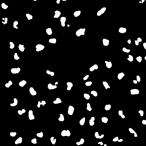
(很明显，这不是相同的图像，但是假设最后一幅图像只是从边缘开始的。)

然后，我想使用类似于computeFeatures()包的EBImage方法(据我所知，这种方法只适用于实体)

Answer 1

编辑更多代码以提取具有“连接”到边框的对象内部。附加代码包括定义分段单元的凸包和创建填充掩码。

简单地说，fillHull和floodFill可能有助于填充具有定义良好边界的单元格。

下面(编辑的)较长的答案表明了一种使用floodFill的方法可能是有用的。你做了一个伟大的工作，从低对比度的DIC图像提取信息，但更多的图像处理可能会有帮助，如“平场校正”对含噪的DIC图像。这个维基百科页面描述了这个原理，但是一个简单的实现会产生奇迹。这里建议的编码解决方案需要用户交互来选择单元格。这不是一种强有力的方法。尽管如此，也许更多的图像处理与代码相结合来定位细胞可能是可行的。最后，对细胞内部进行分割，并利用computeFeatures进行分析。

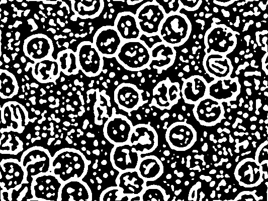
代码从阈值图像开始(对边缘进行修整并转换为二进制)。

# Set up plots for 96 dpi images
  library(EBImage)
  dm <- dim(img2)/96
  dev.new(width = dm[1], height = dm[2])
# Low pass filter with gblur and make binary
  xb <- gblur(img2, 3)
  xt <- thresh(xb, offset = 0.0001)
  plot(xt) # thresh.jpg
# dev.print(jpeg, "thresh.jpg", width = dm[1], unit = "in", res = 96) 

​

​

# Keep only "large" objects
  xm <- bwlabel(xt)
  FS <- computeFeatures.shape(xm)
  sel <- which(FS[,"s.area"] < 800)
  xe <- rmObjects(xm, sel)

# Make binary again and plot
  xe <- thresh(xe)
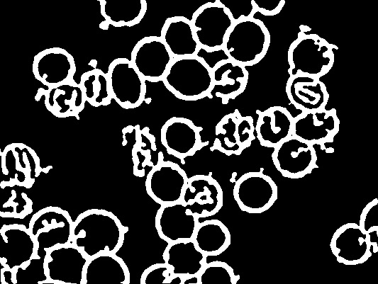
  plot(xe) # trimmed.jpg
#  dev.print(jpeg, "trimmed.jpg", width = dm[1], unit = "in", res = 96)

​

​

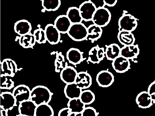
# Choose cells with intact interiors
# This is done by hand here but with more pre-processing, it may be
# possible to have the image suitable for more automated analysis...
  pp <- locator(type = "p", pch = 3, col = 2) # marked.jpg
#  dev.print(jpeg, "marked.jpg", width = dm[1], unit = "in", res = 96)

​

​

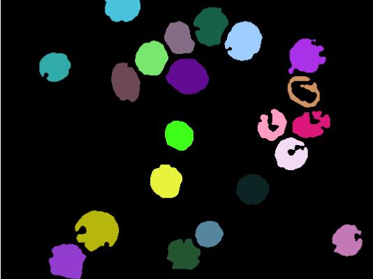
# Fill interior of each cell with a unique integer
  myCol <- seq_along(pp$x) + 1
  xf1 <- floodFill(xe, do.call(rbind, pp), col = myCol)

# Discard original objects from threshold (value = 1) and see
  cells1 <- rmObjects(xf1, 1)
  plot(colorLabels(cells1))
# dev.print(jpeg, "cells1.jpg", width = dm[1], unit = "in", res = 96)

​

​

我需要介绍一些算法来连接顶点之间的整数点，并填充一个凸多边形。这里的代码实现了Bresenham的算法，并使用了一个简单的多边形填充例程，它只适用于凸(简单)多边形。

#
# Bresenham's balanced integer line drawing algorithm
#
bresenham <- function(x, y = NULL, close = TRUE)
{
# accept any coordinate structure
  v <- xy.coords(x = x, y = y, recycle = TRUE, setLab = FALSE)
  if (!all(is.finite(v$x), is.finite(v$y)))
    stop("finite coordinates required")

  v[1:2] <- lapply(v[1:2], round) # Bresenham's algorithm IS for integers
  nx <- length(v$x)
  if (nx == 1) return(list(x = v$x, y = v$y)) # just one point
  if (nx > 2 && close == TRUE) { # close polygon by replicating 1st point
    v$x <- c(v$x, v$x[1])
    v$y <- c(v$y, v$y[1])
    nx <- nx + 1
  }
# collect result in 'ans, staring with 1st point
  ans <- lapply(v[1:2], "[", 1)

# process all vertices in pairs
  for (i in seq.int(nx - 1)) {
    x <- v$x[i] # coordinates updated in x, y
    y <- v$y[i]
    x.end <- v$x[i + 1]
    y.end <- v$y[i + 1]

    dx <- abs(x.end - x); dy <- -abs(y.end - y)
    sx <- ifelse(x < x.end, 1, -1)
    sy <- ifelse(y < y.end, 1, -1)
    err <- dx + dy

  # process one segment
    while(!(isTRUE(all.equal(x, x.end)) && isTRUE(all.equal(y, y.end)))) {
      e2 <- 2 * err
      if (e2 >= dy) { # increment x
        err <- err + dy
        x <- x + sx
      }
      if (e2 <= dx) { # increment y
        err <- err + dx
        y <- y + sy
      }
      ans$x <- c(ans$x, x)
      ans$y <- c(ans$y, y)
    }
  }
# remove duplicated points (typically 1st and last)
  dups <- duplicated(do.call(cbind, ans), MARGIN = 1) 
  return(lapply(ans, "[", !dups))
}

和简单多边形内部点的简单例程。

#
# Return x,y integer coordinates of the interior of a CONVEX polygon
#
cPolyFill <- function(x, y = NULL) 
{
  p <- xy.coords(x, y = y, recycle = TRUE, setLab = FALSE)
  p[1:2] <- lapply(p[1:2], round)
  nx <- length(p$x)
  if (any(!is.finite(p$x), !is.finite(p$y)))
    stop("finite coordinates are needed")

  yc <- seq.int(min(p$y), max(p$y))
  xlist <- lapply(yc, function(y) sort(seq.int(min(p$x[p$y == y]), max(p$x[p$y == y]))))
  ylist <- Map(rep, yc, lengths(xlist))
  ans <- cbind(x = unlist(xlist), y = unlist(ylist))
  return(ans)
}

现在，这些可以与ocontour()和chull()一起使用来创建和填充每个分段单元的凸包。这种“修复”那些细胞的入侵。

# Create convex hull mask
  oc <- ocontour(cells1) # for all points along perimeter
  oc <- lapply(oc, function(v) v + 1) # off-by-one flaw in ocontour
  sel <- lapply(oc, chull) # find points that define convex hull
  xh <- Map(function(v, i) rbind(v[i,]), oc, sel) # new vertices for convex hull
  oc2 <- lapply(xh, bresenham) # perimeter points along convex hull

# Collect interior coordinates and fill
  coords <- lapply(oc2, cPolyFill)
  cells2 <- Image(0, dim = dim(cells1))
  for(i in seq_along(coords))
    cells2[coords[[i]]] <- i # blank image for mask
  xf2 <- xe
  for (i in seq_along(coords))
    xf2[coords[[i]]] <- i # early binary mask

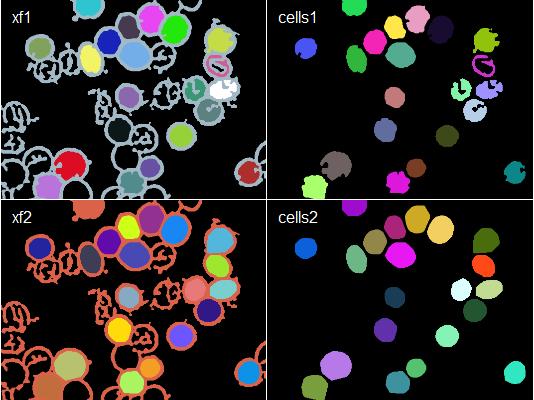
# Compare before and after
  img <- combine(colorLabels(xf1), colorLabels(cells1),
    colorLabels(xf2), colorLabels(cells2))
  plot(img, all = T, nx = 2)
  labs <- c("xf1", "cells1", "xf2", "cells2")
  ix <- c(0, 1, 0, 1)
  iy <- c(0, 0, 1, 1)
  text(dm[1]*96*(ix + 0.05), 96*dm[2]*(iy + 0.05), labels = labs,
    col = "white", adj = c(0.05,1))
 # dev.print(jpeg, "final.jpg", width = dm[1], unit = "in", res = 96)

​

​