智能峰值检测方法

Question

我想使用python从这些数据中检测出峰值：

data = [1.0, 0.35671858559485703, 0.44709399319470694, 0.29438948200831194, 0.5163825635166547, 0.3036363865322419, 0.34031782308777747, 0.2869558046065574, 0.28190537831716, 0.2807516154537239, 0.34320479518313507, 0.21117275536958913, 0.30304626765388043, 0.4972542099530442, 0.0, 0.0, 0.0, 0.0, 0.0, 0.0, 0.0, 0.0, 0.0, 0.0, 0.0, 0.0, 0.0, 0.0, 0.0, 0.0, 0.0, 0.0, 0.0, 0.0, 0.0, 0.0, 0.0, 0.0, 0.0, 0.0, 0.0, 0.0, 0.0, 0.0, 0.0, 0.0, 0.0, 0.0, 0.0, 0.0, 0.0, 0.0, 0.0, 0.0, 0.0, 0.0, 0.0, 0.0, 0.18200891715227194, 0.0, 0.0, 0.0, 0.0, 0.0, 0.0, 0.0, 0.0, 0.0, 0.0, 0.0, 0.0, 0.0, 0.0, 0.0, 0.0, 0.0, 0.0, 0.0, 0.0, 0.0, 0.0, 0.0, 0.0, 0.0, 0.0, 0.0, 0.0, 0.0, 0.0, 0.0, 0.0, 0.0, 0.0, 0.0, 0.0, 0.0, 0.0, 0.0, 0.0, 0.0, 0.0, 0.0, 0.0, 0.0, 0.0, 0.0, 0.0, 0.0, 0.0, 0.0, 0.0, 0.0, 0.0, 0.0, 0.0, 0.0, 0.0, 0.0, 0.0, 0.0, 0.0, 0.0, 0.28830608331168983, 0.057156776746163526, 0.043418555819326035, 0.022527521866967784, 0.035414574439784685, 0.062273775107322626, 0.04569227783752021, 0.04978915781132807, 0.0599089458581528, 0.05692515997545401, 0.05884619933405206, 0.0809943356922021, 0.07466587894671428, 0.08548458657792352, 0.049216679971411645, 0.04742180324984401, 0.05822208549398862, 0.03465282733964001, 0.014005094192867372, 0.052004161876744344, 0.061297263734617496, 0.01867087951563289, 0.01390993522118277, 0.021515814095838564, 0.025260618727204275, 0.0157022555745128, 0.041999490119172936, 0.0441231248537558, 0.03079711140612242, 0.04177946154195037, 0.047476050325192885, 0.05087930020034335, 0.03889899267688956, 0.02114033158686702, 0.026726959895528927, 0.04623461918879543, 0.05426474524591766, 0.04421866212189775, 0.041911901968304605, 0.019982199103543322, 0.026520396430805435, 0.03952286472888431, 0.03842652984978244, 0.02779682035551695, 0.02043518392128019, 0.07706934170969436]

你可以画出来：

import matplotlib.pyplot as plt
plt.plot(data)

​

​

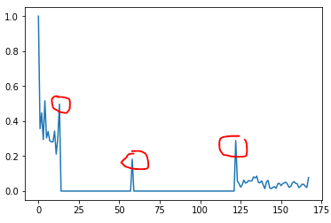
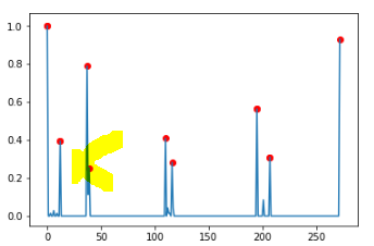
我包围了我想要用红色自动探测到的山峰。

峰特征：

我感兴趣的是找出峰值，然后，对于一些数据点(即3-4)，信号是相对平滑的。平滑的意思是，振幅的变化在峰值后的数据点之间是可比较的。我猜，这在更多的数学术语中意味着:峰值，在此之后，对于一些数据点，如果你拟合一条线性线，那么斜率将接近于0。

到目前为止，我已经尝试过：

我认为元素之间的差异(附加0以具有相同的长度)会更好地显示峰值：

diff_list = []
# Append 0 to have the same length as data 
data_d = np.append(data,0)

for i in range(len(data)):
    diff = data_d[i]-data_d[i+1]

    # If difference is samller than 0, I set it to 0 -> Just interested in "falling" peaks
    if diff < 0:
        diff = 0

    diff_list= np.append(diff_list,diff)

当我绘制diff_list时，它看起来已经好多了：

​

​

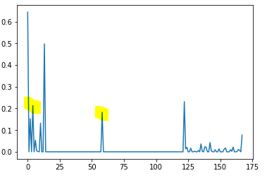
然而，一个简单的阈值峰值检测算法不能工作，因为噪声在第一段有相同的幅度与峰值后。

因此，我需要一种算法，它将可靠地找到峰值，或者一种方法，在不对峰值进行很大阻尼的情况下，大幅降低噪声，最重要的是不移动它们。有人有主意吗?

编辑1:

我偶然发现了这个博客并尝试了这方法：

peaks_d = detect_peaks(diff_list, mph=None, mpd=4, threshold=0.1, edge='falling', kpsh=False, valley=False, show=False, ax=None)
plt.plot(diff_list)
plt.plot(peaks_d[:-1], diff_list[peaks_d[:-1]], "x")
plt.show()

我得到了...but：

​

​

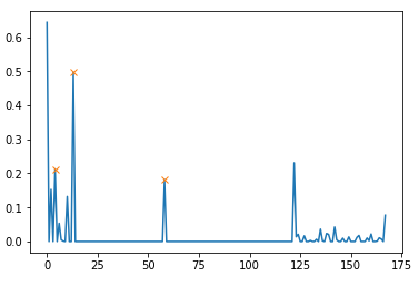
...so说真的，我认为我需要更多的预处理.

编辑2:

所以我试着计算梯度：

plt.plot(np.gradient(data))

不过，噪音内的梯度可与其中一个峰值相比较：

​

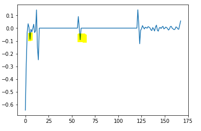
可以使用的是：

->噪声:在一个相邻的位置有许多相似的振幅点。也许可以检测到这些区域并过滤掉它们(即将它们设置为0)。

编辑3:

我试着跟踪这种方法

# Data
y = diff_list.tolist()

# Settings: lag = 30, threshold = 5, influence = 0
lag = 10
threshold = 0.1
influence = 1

# Run algo with settings from above
result = thresholding_algo(y, lag=lag, threshold=threshold, influence=influence)

# Plot result
plt.plot(result["signals"])

然而，我得到：

​

​

编辑4:

基于@Jussi Nurminen的评论：

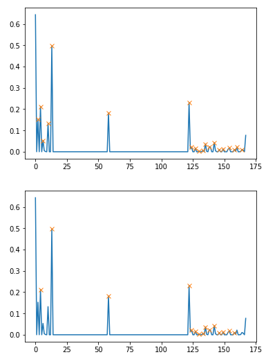
计算导数的绝对值，对峰值后的一些样本进行平均值，看看得到的值是否“足够小”。当然，你必须首先检测所有候选峰。为此，您可以使用scipy.signal.argrelextrema来检测所有本地最大值。

import scipy.signal as sg
max_places = (np.array(sg.argrelmax(diff_list))[0]).tolist()
plt.plot(diff_list)
plt.plot(max_places, diff_list[max_places], "x")
plt.show()

peaks = []
for check in max_places:
    if check+5 < len(diff_list):
        gr = abs(np.average(np.gradient(diff_list[check+1: check+5])))
        if gr < 0.01:
            peaks.append(check)

plt.plot(diff_list)
plt.plot(peaks[:-1], diff_list[peaks[:-1]], "x")
plt.show()

​

​

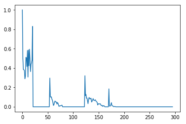
编辑5:

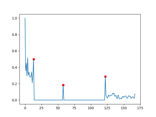
下面是测试任何算法的类似数据：

data2 = [1.0, 0.4996410902399043, 0.3845950995707942, 0.38333441505960125, 0.3746384799687852, 0.28956967636700215, 0.31468441185494306, 0.5109048238958792, 0.5041481423190644, 0.41629226772762024, 0.5817609846838199, 0.3072152962171569, 0.5870564826981163, 0.4233247394608264, 0.5943712016644392, 0.4946091070102793, 0.36316740988182716, 0.4387555870158762, 0.45290920032442744, 0.48445358617984213, 0.8303387875295111, 0.0, 0.0, 0.0, 0.0, 0.0, 0.0, 0.0, 0.0, 0.0, 0.0, 0.0, 0.0, 0.0, 0.0, 0.0, 0.0, 0.0, 0.0, 0.0, 0.0, 0.0, 0.0, 0.0, 0.0, 0.0, 0.0, 0.0, 0.0, 0.0, 0.0, 0.0, 0.0, 0.0, 0.29678306715530073, 0.10146278147135124, 0.10120143287506084, 0.10330143251114839, 0.0802259786323741, 0.06858944745608002, 0.04600545347437729, 0.014440053029463367, 0.019023393725625705, 0.045201054387436344, 0.058496635702267374, 0.05656947149500993, 0.0463696266116956, 0.04903205756575247, 0.02781307505224703, 0.044280150764466876, 0.03746976646628557, 0.021526918040025544, 0.0038244080425488013, 0.008617907527160991, 0.0112760689575489, 0.009157686770957874, 0.013043259260489413, 0.01621417695776057, 0.016502269315028423, 0.0, 0.0, 0.0, 0.0, 0.0, 0.0, 0.0, 0.0, 0.0, 0.0, 0.0, 0.0, 0.0, 0.0, 0.0, 0.0, 0.0, 0.0, 0.0, 0.0, 0.0, 0.0, 0.0, 0.0, 0.0, 0.0, 0.0, 0.0, 0.0, 0.0, 0.0, 0.0, 0.0, 0.0, 0.0, 0.0, 0.0, 0.0, 0.0, 0.0, 0.0, 0.0, 0.0, 0.0, 0.3210019708643843, 0.11441868790191953, 0.12862935834434436, 0.08790971283197381, 0.09127615787146504, 0.06360039847679771, 0.032247149009635476, 0.07225952295002563, 0.095632185243862, 0.09171396569135751, 0.07935726217072689, 0.08690487354356599, 0.08787369092132288, 0.04980466729311508, 0.05675819557118429, 0.06826614158574265, 0.08491084598657253, 0.07037944101030547, 0.06549710463329293, 0.06429902857281444, 0.07282805735716101, 0.0667027178198566, 0.05590329380937183, 0.05189048980041104, 0.04609913889901785, 0.01884014489167378, 0.02782496113905073, 0.03343588833365329, 0.028423168106849694, 0.028895130687196867, 0.03146961123393891, 0.02287127937400026, 0.012173655214339595, 0.013332601407407033, 0.014040309216796854, 0.003450677642354792, 0.010854992025496528, 0.011804042414950701, 0.008100266690771957, 0.0, 0.0, 0.0, 0.0, 0.0, 0.0, 0.0, 0.0, 0.18547803170164875, 0.008457776819382444, 0.006607607749756658, 0.008566964920042127, 0.024793283595437438, 0.04334031667011553, 0.012330921737457376, 0.00994343436054472, 0.008003962298473758, 0.0025523166577987263, 0.0009309499302016907, 0.0027602202618852126, 0.0034442123857338675, 0.0006448449815386562, 0.0, 0.0, 0.0, 0.0, 0.0, 0.0, 0.0, 0.0, 0.0, 0.0, 0.0, 0.0, 0.0, 0.0, 0.0, 0.0, 0.0, 0.0, 0.0, 0.0, 0.0, 0.0, 0.0, 0.0, 0.0, 0.0, 0.0, 0.0, 0.0, 0.0, 0.0, 0.0, 0.0, 0.0, 0.0, 0.0, 0.0, 0.0, 0.0, 0.0, 0.0, 0.0, 0.0, 0.0, 0.0, 0.0, 0.0, 0.0, 0.0, 0.0, 0.0, 0.0, 0.0, 0.0, 0.0, 0.0, 0.0, 0.0, 0.0, 0.0, 0.0, 0.0, 0.0, 0.0, 0.0, 0.0, 0.0, 0.0, 0.0, 0.0, 0.0, 0.0, 0.0, 0.0, 0.0, 0.0, 0.0, 0.0, 0.0, 0.0, 0.0, 0.0, 0.0, 0.0, 0.0, 0.0, 0.0, 0.0, 0.0, 0.0, 0.0, 0.0, 0.0, 0.0, 0.0, 0.0, 0.0, 0.0, 0.0, 0.0, 0.0, 0.0, 0.0, 0.0, 0.0, 0.0, 0.0, 0.0, 0.0, 0.0, 0.0, 0.0]

​

​

使用@jojo的答案，并选择适当的参数(dy_lim = 0.1和di_lim = 10 )，结果是接近的，但是添加了一些不应该是峰值的点。

​

​

编辑5:

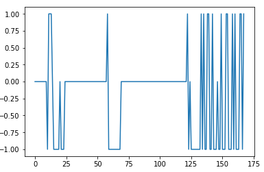
不过，又是个案子。

data = [1.0, 0.0, -0.0, 0.014084507042253521, 0.0, -0.0, 0.028169014084507043, 0.0, -0.0, 0.014084507042253521, 0.0, 0.0, 0.39436619718309857, -0.0, -0.0, -0.0, -0.0, -0.0, -0.0, -0.0, -0.0, -0.0, -0.0, -0.0, -0.0, -0.0, -0.0, -0.0, -0.0, -0.0, -0.0, -0.0, -0.0, -0.0, -0.0, -0.0, 0.0, 0.7887323943661971, 0.11267605633802817, 0.2535211267605634, -0.0, -0.0, -0.0, -0.0, -0.0, -0.0, -0.0, -0.0, -0.0, -0.0, -0.0, -0.0, -0.0, -0.0, -0.0, -0.0, -0.0, -0.0, -0.0, -0.0, -0.0, -0.0, -0.0, -0.0, -0.0, -0.0, -0.0, -0.0, -0.0, -0.0, -0.0, -0.0, -0.0, -0.0, -0.0, -0.0, -0.0, -0.0, -0.0, -0.0, -0.0, -0.0, -0.0, -0.0, -0.0, -0.0, -0.0, -0.0, -0.0, -0.0, -0.0, -0.0, -0.0, -0.0, -0.0, -0.0, -0.0, -0.0, -0.0, -0.0, -0.0, -0.0, -0.0, -0.0, -0.0, -0.0, -0.0, -0.0, -0.0, 0.0, 0.4084507042253521, -0.0, 0.04225352112676056, 0.014084507042253521, 0.014084507042253521, 0.0, 0.28169014084507044, 0.04225352112676056, -0.0, -0.0, -0.0, -0.0, -0.0, -0.0, -0.0, -0.0, -0.0, -0.0, -0.0, -0.0, -0.0, -0.0, -0.0, -0.0, -0.0, -0.0, -0.0, -0.0, -0.0, -0.0, -0.0, -0.0, -0.0, -0.0, -0.0, -0.0, -0.0, -0.0, -0.0, -0.0, -0.0, -0.0, -0.0, -0.0, -0.0, -0.0, -0.0, -0.0, -0.0, -0.0, -0.0, -0.0, -0.0, -0.0, -0.0, -0.0, -0.0, -0.0, -0.0, -0.0, -0.0, -0.0, -0.0, -0.0, -0.0, -0.0, -0.0, -0.0, -0.0, -0.0, -0.0, -0.0, -0.0, -0.0, -0.0, -0.0, -0.0, -0.0, -0.0, -0.0, -0.0, -0.0, -0.0, -0.0, 0.0, 0.5633802816901409, -0.0, -0.0, -0.0, -0.0, 0.0, 0.08450704225352113, -0.0, -0.0, -0.0, -0.0, 0.0, 0.30985915492957744, -0.0, -0.0, -0.0, -0.0, -0.0, -0.0, -0.0, -0.0, -0.0, -0.0, -0.0, -0.0, -0.0, -0.0, -0.0, -0.0, -0.0, -0.0, -0.0, -0.0, -0.0, -0.0, -0.0, -0.0, -0.0, -0.0, -0.0, -0.0, -0.0, -0.0, -0.0, -0.0, -0.0, -0.0, -0.0, -0.0, -0.0, -0.0, -0.0, -0.0, -0.0, -0.0, -0.0, -0.0, -0.0, -0.0, -0.0, -0.0, -0.0, -0.0, -0.0, -0.0, -0.0, -0.0, -0.0, -0.0, -0.0, -0.0, -0.0, -0.0, -0.0, -0.0, -0.0, 0.0, 0.9295774647887324]

​

​

在这里，几乎所有的峰值都被正确地检测到，只有一个。

Answer 1

这是一个务实的解决方案，正如我所看到的(如果我错了请纠正我)，您希望在“平稳”或“0”周期之后/之前找到每个峰值。

您可以通过简单地检查这些时间段并报告它们的开始和停止来做到这一点。

下面是一个非常基本的实现，允许指定什么是smooth期间(这里我使用小于0.001的更改作为条件)：

dy_lim = 0.001
targets = []
in_lock = False
i_l, d_l = 0, data[0]
for i, d in enumerate(data[1:]):
    if abs(d_l - d) > dy_lim:
        if in_lock:
            targets.append(i_l)
            targets.append(i + 1)
            in_lock = False
        i_l, d_l = i, d
    else:
        in_lock = True

然后绘制targets

plt.plot(range(len(data)), data)
plt.scatter(targets, [data[t] for t in targets], c='red')
plt.show()

​

​

没有什么非常详细的，但它找到了你指出的峰值。

增加dy_lim的值将使您找到更多的峰值。另外，您可能希望指定一个平滑周期的最小长度，下面是这个过程的样子(同样只是一个粗略的实现)：

dy_lim = 0.001
di_lim = 50
targets = []
in_lock = False
i_l, d_l = 0, data[0]
for i, d in enumerate(data[1:]):
    if abs(d_l - d) > dy_lim:
        if in_lock:
            in_lock = False
            if i - i_l > di_lim:
                targets.append(i_l)
                targets.append(i + 1)
        i_l, d_l = i, d
    else:
        in_lock = True

有了这个，你就不会得到第一个点，因为第一和第二之间的差异大于di_lim=50。

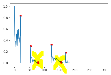
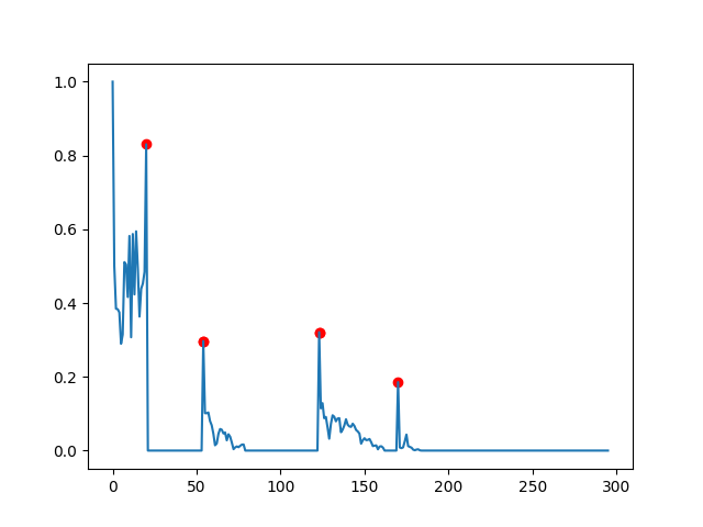
第二个数据集的更新：

这变得更加棘手，因为现在在峰值后逐渐减少，导致差异的缓慢聚集，足以击中dy_lim，导致算法错误地报告一个新的目标。因此，，您需要测试这个目标是否真的是一个峰值，并且只报告。

以下是如何实现这一目标的粗略实现：

dy_lim = 0.1
di_lim = 5
targets = []
in_lock = False
i_l, d_l = 0, data[0]
for i, d in enumerate(data[1:]):
    if abs(d_l - d) > dy_lim:
        if in_lock:
            in_lock = False
            if i - i_l > di_lim:
                # here we check whether the start of the period was a peak
                if abs(d_l - data[i_l]) > dy_lim:
                    # assure minimal distance if previous target exists
                    if targets:
                        if i_l - targets[-1] > di_lim:
                            targets.append(i_l)
                    else:
                        targets.append(i_l)
                # and here whether the end is a peak
                if abs(d - data[i]) > dy_lim:
                    targets.append(i + 1)
        i_l, d_l = i, d
    else:
        in_lock = True

你最终会得到的是：

​

一般注意:我们在这里遵循一种自下而上的方法:您有一个要检测的特定特性，所以您需要编写一个特定的算法。

这对于简单的任务是非常有效的，但是在这个简单的例子中，我们已经意识到，如果有新的特征，算法应该能够处理，我们需要适应它。如果只有当前的复杂性，那么您就没事了。但是，如果数据出现了其他模式，那么您将再次遇到需要添加更多条件的情况，算法将变得越来越复杂，因为它需要处理额外的复杂性。如果你在这样的情况下结束，那么你可能想要考虑切换，并适应一种更真实的方法。在这种情况下，有许多选项，一种方法是使用萨维斯基-戈莱过滤版本处理原始数据的差异，但这只是在这里可以提出的许多建议之一。

Answer 2

您可能需要尝试scipy.signal.find_peaks，它允许您指定不同的标准(突出度、宽度、高度等)。但是，您首先必须弄清楚您的“高峰”标准是什么。仅仅说你想要一些峰值，而不是其他一些峰值是不够的--它们之间必须有一些差异，这是算法能够检测到的。