ggridges直方图下的阴影面积(stat = binline)？

Question

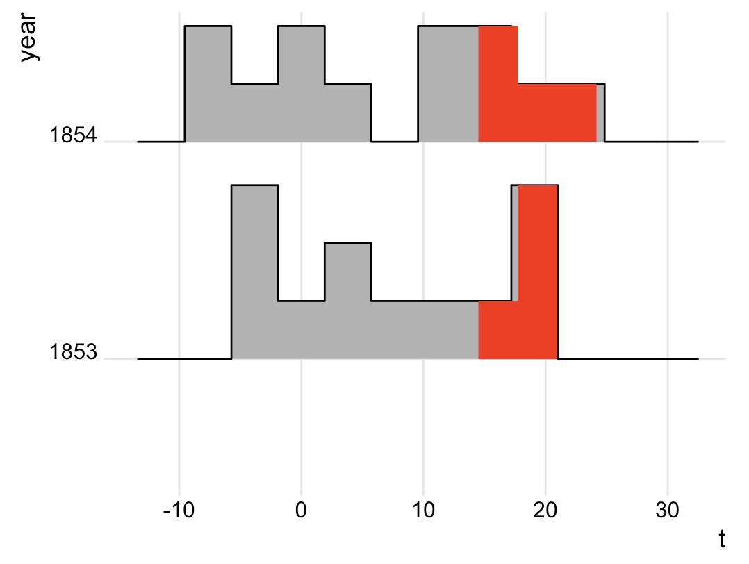
使用Evers suggestion博士在密度曲线下用ggridges对区域进行遮阳效果很好。然而，我发现密度曲线可能具有欺骗性，因为它们意味着数据在没有数据的情况下存在。因此，我想我应该用普通的直方图来尝试这种阴影技术。

然而，当我试图使用它与直方图，阴影是有点差。为什么会这样呢？

library(tidyverse)
install.packages("ggridges", dependencies=TRUE)  # there are many
library(ggridges)
 t2 <-   structure(list(Date = c("1853-01", "1853-02", "1853-03", "1853-04", 
"1853-05", "1853-06", "1853-07", "1853-08", "1853-09", "1853-10", 
"1853-11", "1853-12", "1854-01", "1854-02", "1854-03", "1854-04", 
"1854-05", "1854-06", "1854-07", "1854-08", "1854-09", "1854-10", 
"1854-11", "1854-12"), t = c(-5.6, -5.3, -1.5, 4.9, 9.8, 17.9, 
18.5, 19.9, 14.8, 6.2, 3.1, -4.3, -5.9, -7, -1.3, 4.1, 10, 16.8, 
22, 20, 16.1, 10.1, 1.8, -5.6), year = c("1853", "1853", "1853", 
"1853", "1853", "1853", "1853", "1853", "1853", "1853", "1853", 
"1853", "1854", "1854", "1854", "1854", "1854", "1854", "1854", 
"1854", "1854", "1854", "1854", "1854")), row.names = c(NA, -24L
), class = c("tbl_df", "tbl", "data.frame"), .Names = c("Date", 
"t", "year"))


gg <- ggplot(t2, aes(x = t, y = year)) +
      geom_density_ridges(stat = "binline", bins = 10, scale = 0.8, 
                      draw_baseline = TRUE) +
      theme_ridges()

# Build ggplot and extract data
d <- ggplot_build(gg)$data[[1]]

# Add geom_ribbon for shaded area
gg +
  geom_ribbon(
    data = transform(subset(d, x >= 10), year = group),
    aes(x, ymin = ymin, ymax = ymax, group = group),
    fill = "red",
    alpha = 1.0) 

​

​

Answer 1

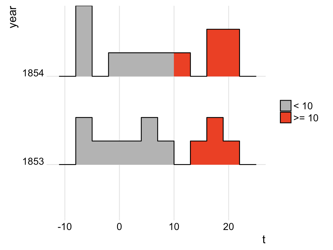
下面的工作，如果你愿意调整大小和移动垃圾箱，所以一个垃圾箱边界正好在你的分界线(这里10)。

ggplot(t2, aes(x = t, y = year, fill = ifelse(..x..>=10, ">= 10", "< 10"))) +
  geom_density_ridges_gradient(stat = "binline", binwidth = 3,
                               center = 8.5, scale = 0.8, 
                               draw_baseline = TRUE) +
  theme_ridges() +
  scale_fill_manual(values = c("gray70", "red"), name = NULL)

​

​

您之所以观察到所做的效果，是因为x轴在第一幅和第二幅图之间发生了变化，而x轴范围对如何绘制回收箱产生了影响。有两种解决方案:要么修复x轴范围，要么通过center和binwidth定义回收箱，而不是通过bins。(在我看来，无论你如何对待x轴，第二种选择总是可取的。)

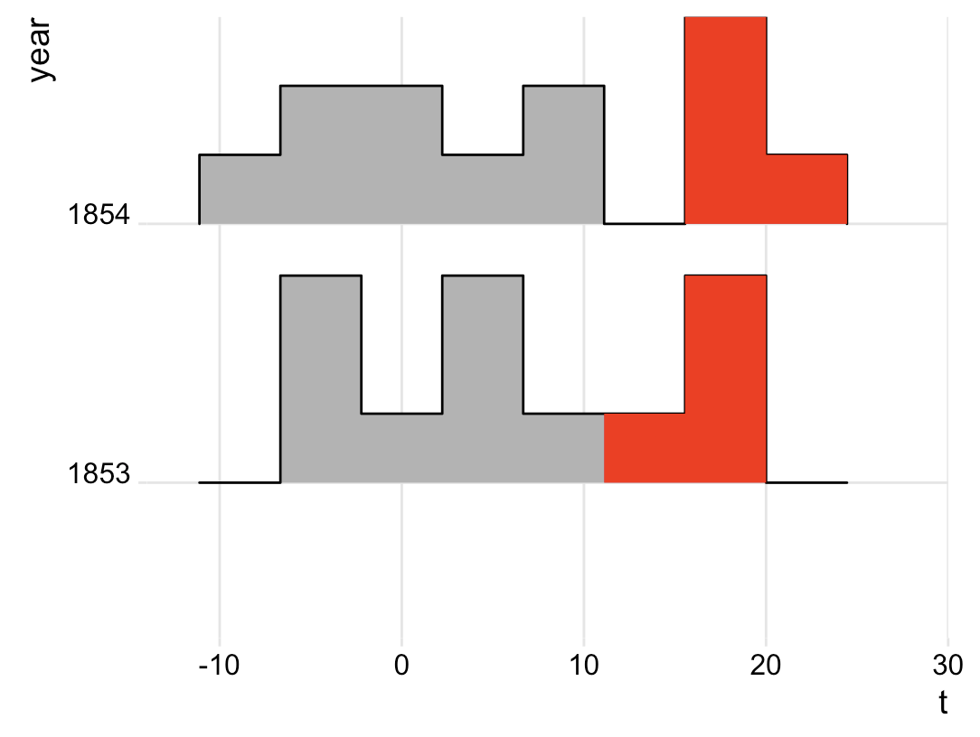
首先，修复x轴范围：

gg <- ggplot(t2, aes(x = t, y = year)) +
  geom_density_ridges(stat = "binline", bins = 10, scale = 0.8, 
                      draw_baseline = TRUE) +
  theme_ridges() +
  scale_x_continuous(limits = c(-12, 28)) # this is where the change is

# Build ggplot and extract data
d <- ggplot_build(gg)$data[[1]]

# Add geom_ribbon for shaded area
gg +
  geom_ribbon(
    data = transform(subset(d, x >= 10), year = group),
    aes(x, ymin = ymin, ymax = ymax, group = group),
    fill = "red",
    alpha = 1.0) 

​

​

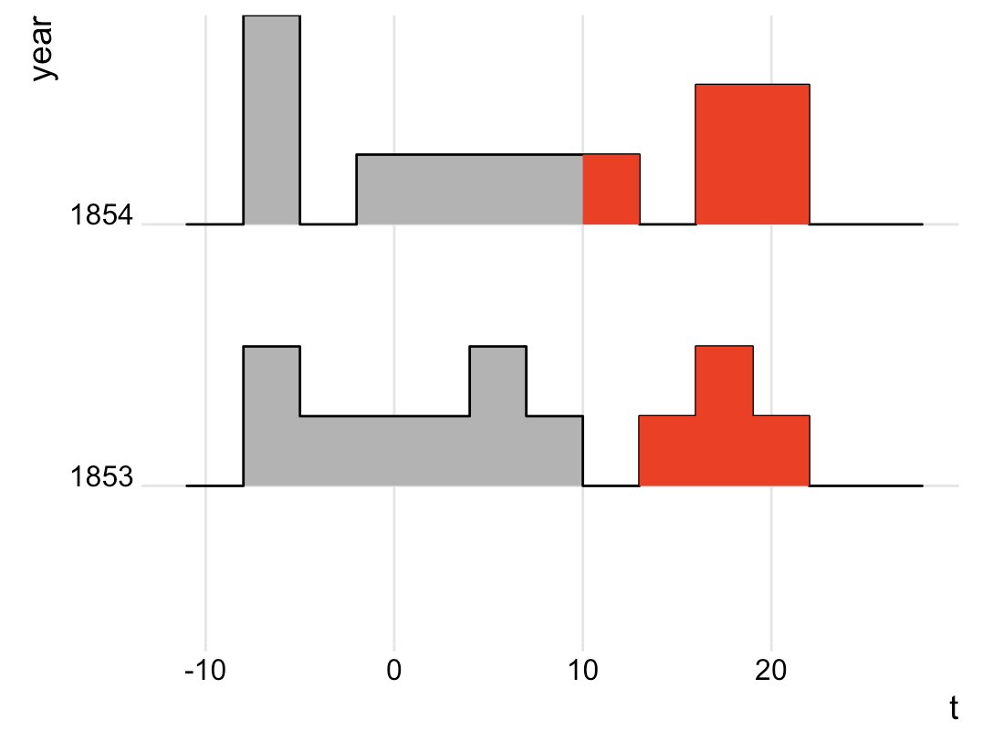
第二，另一种垃圾桶定义：

gg <- ggplot(t2, aes(x = t, y = year)) +
  geom_density_ridges(stat = "binline",
                      binwidth = 3, center = 8.5, # this is where the change is
                      scale = 0.8, draw_baseline = TRUE) +
  theme_ridges()

# Build ggplot and extract data
d <- ggplot_build(gg)$data[[1]]

# Add geom_ribbon for shaded area
gg +
  geom_ribbon(
    data = transform(subset(d, x >= 10), year = group),
    aes(x, ymin = ymin, ymax = ymax, group = group),
    fill = "red",
    alpha = 1.0) 

​

​

Answer 2

确实发生了一些奇怪的事情。关于“结论”，请见下文。

1. 如果我们只绘制gg： gg；

​

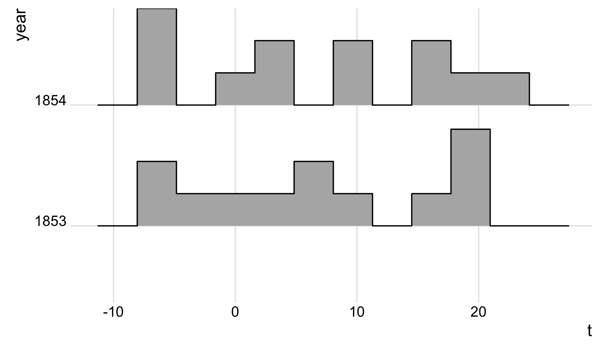
1. 如果我们绘制gg，再加上一个与gg跟踪相对应的楼梯： gg + geom_step( data = d，aes(xmax，ymax，group = group)，方向= "vh"，col = "red"，size = 2)；

​

​

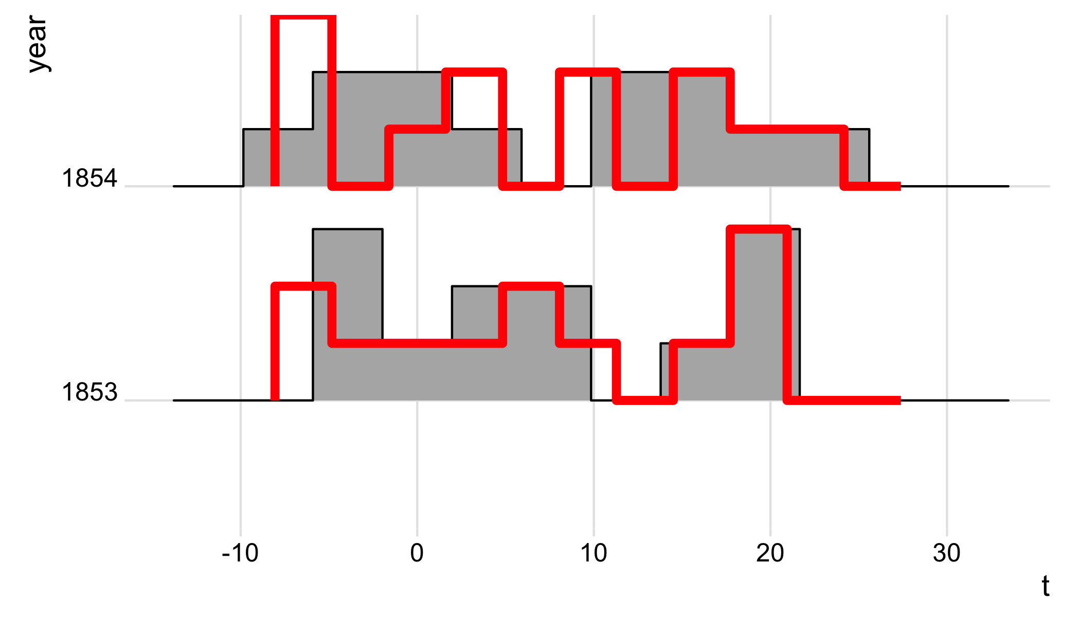
因此，添加geom_step 会改变 gg**.我不明白这怎么可能。您可以看到，** geom_step (红色曲线)在自行绘制 gg 时实际上与直方图的跟踪相对应(见第一幅图)。