pykalman：(默认)处理缺失的值

Question

我正在使用来自pykalman模块的KalmanFilter，并且想知道它是如何处理丢失的观测的。根据文件：

在现实世界中，传感器偶尔失效是很常见的。Kalman滤波器、Kalman平滑器和EM算法都具备处理这种情况的能力。要使用它，只需在缺少的时间步骤中将NumPy掩码应用于度量： 从numpy导入ma X= ma.array(1,2,3) X1 = ma.masked #隐藏时间步骤1 kf.em(X).smooth(X)

我们可以平滑输入时间序列。由于这是一个“附加”函数，我假设它不是自动完成的；那么，当变量中有NaNs时，默认的方法是什么？

这里解释了一种可能发生的理论方法；这也是pykalman所做的事情(在我看来，这将是非常棒的)：

交叉验证-如何处理不完整的数据在卡尔曼滤波？

Answer 1

让我们看一下源代码：

在filter_update函数中，pykalman检查当前的观察是否被屏蔽。

def filter_update(...)

        # Make a masked observation if necessary
        if observation is None:
            n_dim_obs = observation_covariance.shape[0]
            observation = np.ma.array(np.zeros(n_dim_obs))
            observation.mask = True
        else:
            observation = np.ma.asarray(observation) 

它不影响预测步骤。但调整步骤有两种选择。它发生在_filter_correct函数中。

def _filter_correct(...)

    if not np.any(np.ma.getmask(observation)):

         # the normal Kalman Filter math

    else:
        n_dim_state = predicted_state_covariance.shape[0]
        n_dim_obs = observation_matrix.shape[0]
        kalman_gain = np.zeros((n_dim_state, n_dim_obs))

        # !!!! the corrected state takes the result of the prediction !!!!

        corrected_state_mean = predicted_state_mean
        corrected_state_covariance = predicted_state_covariance

正如你所看到的，这正是理论上的方法。

这里有一个简短的示例和工作数据可供使用。

假设你有一个gps接收器，你想在走路的时候跟踪自己。该接收器具有很好的精度。为了简化，假设你只向前走。

​

​

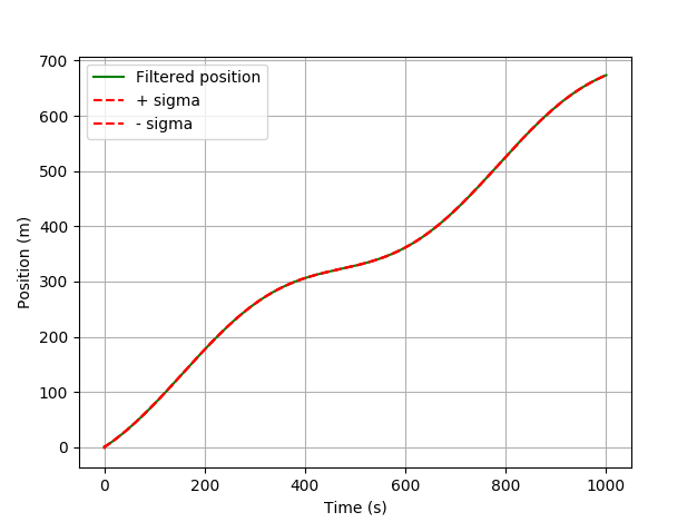
没什么有趣的事。滤波器很好地估计你的位置，因为有一个好的gps信号。如果你有一段时间没有信号怎么办？

​

​

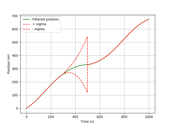
该滤波器只能根据现有状态和系统动力学知识进行预测(，参见矩阵Q，)。随着预测的每一步，不确定性都在增加。估计位置周围的1西格玛范围越来越大.一旦新的观察再次出现，状态就会得到纠正。

下面是代码和数据

from pykalman import KalmanFilter
import numpy as np
import matplotlib.pyplot as plt
from numpy import ma

# enable or disable missing observations
use_mask = 1

# reading data (quick and dirty)
Time=[]
X=[]

for line in open('data/dataset_01.csv'):
    f1, f2  = line.split(';')
    Time.append(float(f1))
    X.append(float(f2))

if (use_mask):
    X = ma.asarray(X)
    X[300:500] = ma.masked

# Filter Configuration

# time step
dt = Time[2] - Time[1]

# transition_matrix  
F = [[1,  dt,   0.5*dt*dt], 
     [0,   1,          dt],
     [0,   0,           1]]  

# observation_matrix   
H = [1, 0, 0]

# transition_covariance 
Q = [[   1,     0,     0], 
     [   0,  1e-4,     0],
     [   0,     0,  1e-6]] 

# observation_covariance 
R = [0.04] # max error = 0.6m

# initial_state_mean
X0 = [0,
      0,
      0]

# initial_state_covariance
P0 = [[ 10,    0,   0], 
      [  0,    1,   0],
      [  0,    0,   1]]

n_timesteps = len(Time)
n_dim_state = 3

filtered_state_means = np.zeros((n_timesteps, n_dim_state))
filtered_state_covariances = np.zeros((n_timesteps, n_dim_state, n_dim_state))

# Kalman-Filter initialization
kf = KalmanFilter(transition_matrices = F, 
                  observation_matrices = H, 
                  transition_covariance = Q, 
                  observation_covariance = R, 
                  initial_state_mean = X0, 
                  initial_state_covariance = P0)


# iterative estimation for each new measurement
for t in range(n_timesteps):
    if t == 0:
        filtered_state_means[t] = X0
        filtered_state_covariances[t] = P0
    else:
        filtered_state_means[t], filtered_state_covariances[t] = (
        kf.filter_update(
            filtered_state_means[t-1],
            filtered_state_covariances[t-1],
            observation = X[t])
        )

position_sigma = np.sqrt(filtered_state_covariances[:, 0, 0]);        

# plot of the resulted trajectory        
plt.plot(Time, filtered_state_means[:, 0], "g-", label="Filtered position", markersize=1)
plt.plot(Time, filtered_state_means[:, 0] + position_sigma, "r--", label="+ sigma", markersize=1)
plt.plot(Time, filtered_state_means[:, 0] - position_sigma, "r--", label="- sigma", markersize=1)
plt.grid()
plt.legend(loc="upper left")
plt.xlabel("Time (s)")
plt.ylabel("Position (m)")
plt.show()      

更新

如果你掩盖一个更长的时间(300:700)，那就更有趣了。

​

​

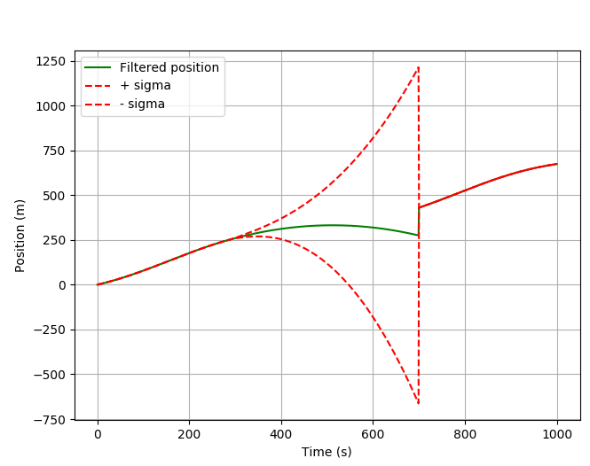
正如你所看到的那样，这个位置又回到了过去。这是由于过渡矩阵F的存在，它将位置、速度和加速度的预测结合起来。

如果你看一下速度状态，它解释了下降的位置。

​

​

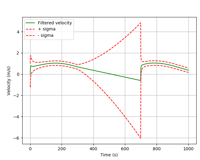
在300秒的时间点，加速度冻结.速度以一个恒定的斜率下降，并越过0值。在这个时间点之后，这个位置必须返回。

要绘制速度图，请使用以下代码：

velocity_sigma = np.sqrt(filtered_state_covariances[:, 1, 1]);     

# plot of the estimated velocity        
plt.plot(Time, filtered_state_means[:, 1], "g-", label="Filtered velocity", markersize=1)
plt.plot(Time, filtered_state_means[:, 1] + velocity_sigma, "r--", label="+ sigma", markersize=1)
plt.plot(Time, filtered_state_means[:, 1] - velocity_sigma, "r--", label="- sigma", markersize=1)
plt.grid()
plt.legend(loc="upper left")
plt.xlabel("Time (s)")
plt.ylabel("Velocity (m/s)")
plt.show()