使用cowplot::plot_grid()时，使用coord_equal()垂直对齐不同高度的绘图

Question

我正在尝试使用cowplot::plot_grid()组合两个ggplot对象，并将它们垂直对齐。使用align = "v"通常非常简单。

dat1 <- data.frame(x = rep(1:10, 2), y = 1:20)
dat2 <- data.frame(x = 1:10, y = 1:10)
plot1 <- ggplot(dat1, aes(x = x, y = y)) + geom_point()
plot2 <- ggplot(dat2, aes(x = x, y = y)) + geom_point()
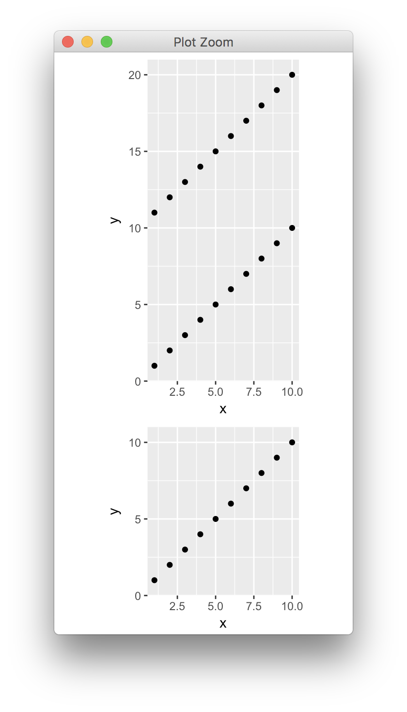
cowplot::plot_grid(plot1, plot2, ncol = 1, align = "v")

​

​

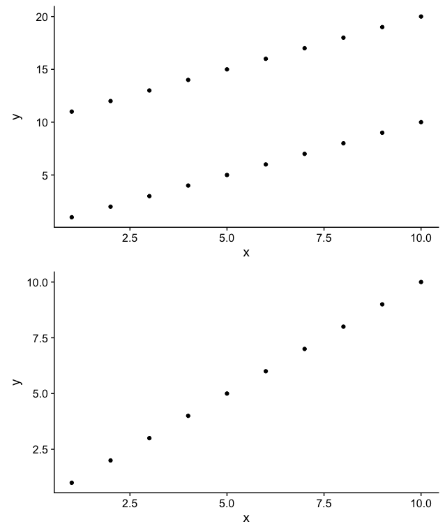
但是，当ggplots使用coord_equal()时，这种方法会失败，因为当高宽比被强制时，plot_grid()无法修改轴。相反，默认的做法是保持每个地块的高度不变。

plot1 <- ggplot(dat1, aes(x = x, y = y)) + geom_point() + coord_equal()
plot2 <- ggplot(dat2, aes(x = x, y = y)) + geom_point() + coord_equal()
cowplot::plot_grid(plot1, plot2, ncol = 1, align = "v")

​

​

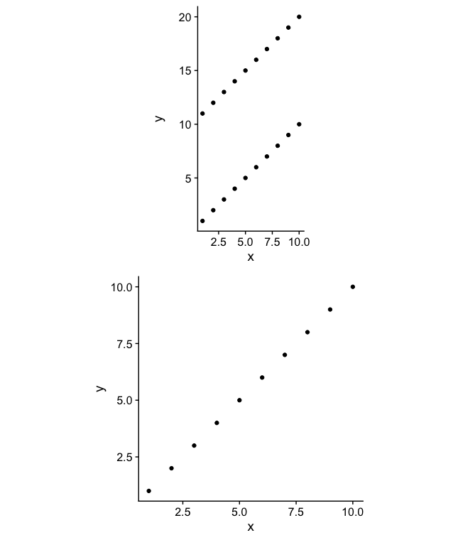
我可以通过正确地处理和获得rel_heights参数来强制我的目标，但是这不是一个可行的解决方案，因为我有很多动态的计划要构建。在这里，y轴是对齐的，所有轴的坐标仍然相等.

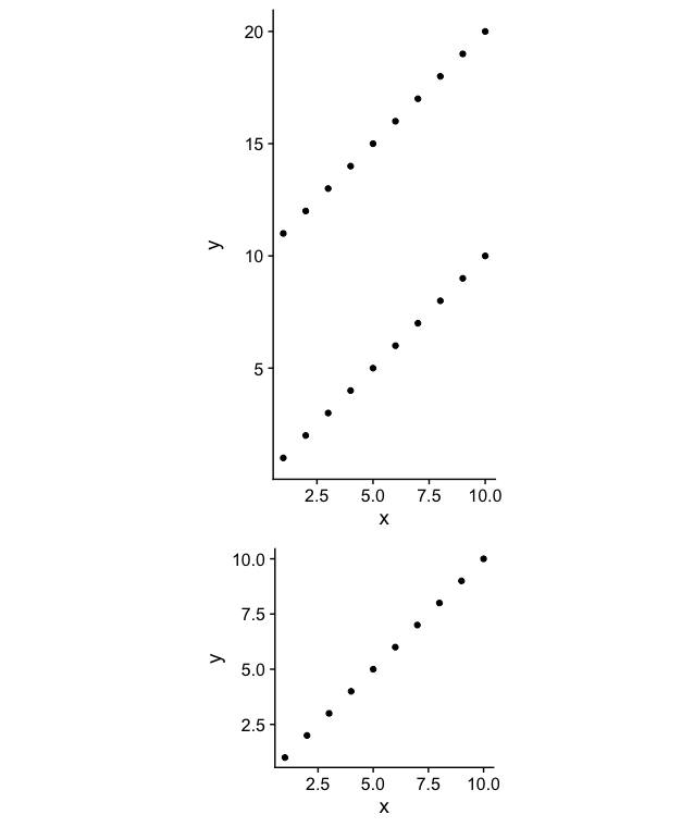
cowplot::plot_grid(plot1, plot2, ncol = 1, align = "v", rel_heights = c(2, 1.07))

​

​

我看到了许多使用ggplot2::ggplotGrob()和grid::grid_draw()来解决类似问题的方法，但是当使用coord_equal()时，没有什么能真正解决这个问题。也许最好的解决方案根本不使用cowplot::plot_grid()，或者解决方案是以某种方式动态地确定并将正确的值传递给rel_heights。我想我更喜欢后面的选项，以便能够轻松地使用cowplot::plot_grid()附带的其他特性。也许可以在这种相关的方法中找到一些有用的启示。

Answer 1

cowplot::plot_grid()的作者。当您试图将图幅与指定的高宽比(当使用coord_equal()时生成)对齐时，它不起作用。解决方案是要么使用鸡蛋库，要么使用拼贴库。拼贴仍在开发中，但很快就会发布。同时，您可以从github安装。

这里有一个使用鸡蛋的解决方案。在我看来它运转得很好。

library(ggplot2)
library(egg)

dat1 <- data.frame(x = rep(1:10, 2), y = 1:20)
dat2 <- data.frame(x = 1:10, y = 1:10)
plot1 <- ggplot(dat1, aes(x = x, y = y)) + geom_point() + coord_equal()
plot2 <- ggplot(dat2, aes(x = x, y = y)) + geom_point() + coord_equal()
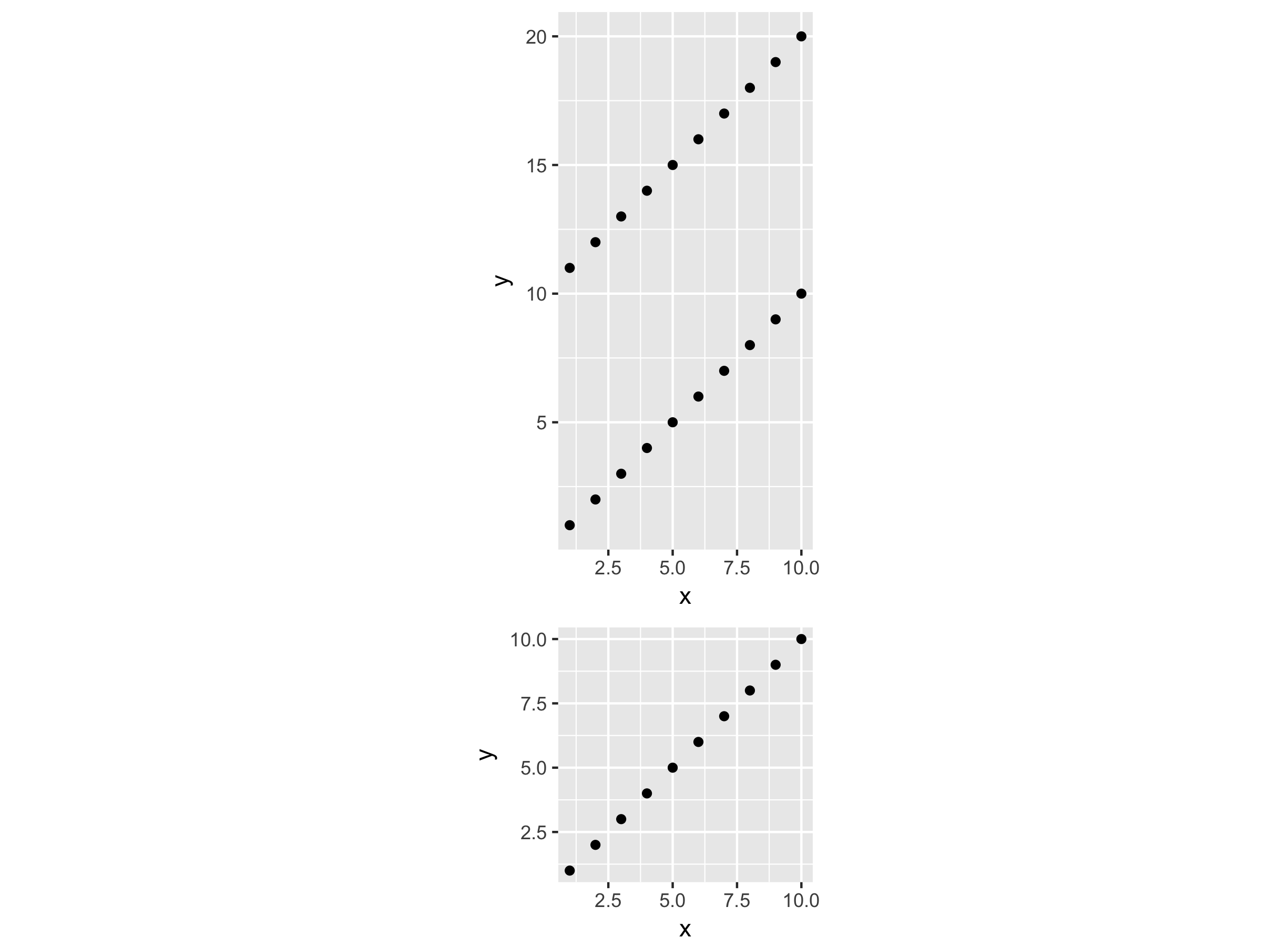
ggarrange(plot1, plot2, ncol = 1)

​

​

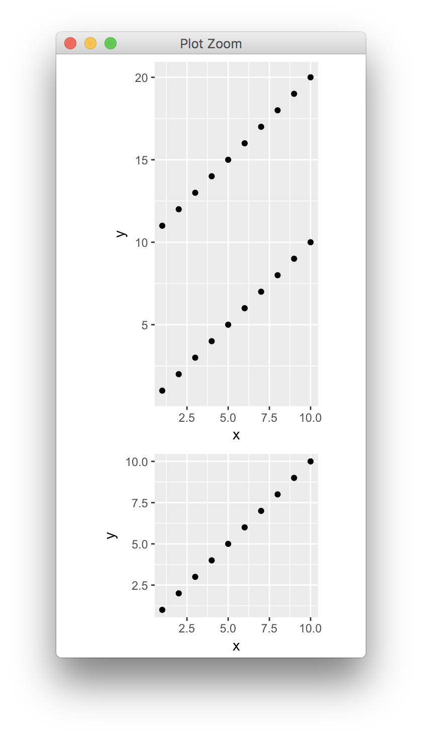
我看到的两个小问题是：(1)两个y轴的轴点是不同的，这使它看起来好像间距不同，(2)轴被扩展到不同的极限。您可以通过手动设置刻度和扩展来解决这两个问题。

plot1 <- ggplot(dat1, aes(x = x, y = y)) + geom_point() + 
  scale_y_continuous(limits = c(0, 21), breaks = 5*(0:4), expand = c(0, 0)) +
  coord_equal()
plot2 <- ggplot(dat2, aes(x = x, y = y)) + geom_point() + 
  scale_y_continuous(limits = c(0, 11), breaks = 5*(0:4), expand = c(0, 0)) +
  coord_equal()
ggarrange(plot1, plot2, ncol = 1)

​

​

Answer 2

默认情况下，这些轴的范围实际上超出了ggplot中的限制。函数scale_continuous/discrete()中的scale_continuous/discrete()参数用于设置扩展。与scale_continuous()文档一样：

长度为2的数值向量，给出乘法和加性展开常数。这些常量确保数据被放置在离轴很远的地方。对于连续变量，默认值为c(0.05，0)，对于离散变量，默认值为c(0，0.6)。

library(ggplot2)
dat1 <- data.frame(x = rep(1:10, 2), y = 1:20)
dat2 <- data.frame(x = 1:10, y = 1:10)
plot1 <- ggplot(dat1, aes(x = x, y = y)) + geom_point() + coord_equal()
plot2 <- ggplot(dat2, aes(x = x, y = y)) + geom_point() + coord_equal()

首先，我们可以计算这两幅图的实际高度，这个职位解释了expand参数是如何工作的。

# The defaults are c(0.05, 0) for your continuous variables
limity1 <- max(dat1$y) - min(dat1$y)
y1 <- limity1 + 2 * limity1 * 0.05
limity2 <- max(dat2$y) - min(dat2$y)
y2 <- limity2 + 2 * limity2 * 0.05

然后，使用拼凑编写这两幅图

library(patchwork)
#  actual heights of plots was used to set the heights argment
plot1 + plot2 + plot_layout(ncol = 1, heights = c(y1, y2))

​

​