问Python OpenCV中的阴影去除
EN

Stack Overflow用户

提问于 2017-12-11 02:07:44

回答 1查看 8.9K关注 0票数 8

我正在尝试使用Finlayson，et的熵最小化方法来实现python OpenCV中的阴影去除。艾尔：

“熵最小化的内在图像”，Finlayson等。阿尔。

我似乎无法与论文的结果相匹配。我的熵图和纸上的不匹配，我得到了错误的最小熵。

有什么想法吗？(根据要求，我有更多的源代码和文件)

#############
# LIBRARIES
#############
import numpy as np
import cv2
import os
import sys
import matplotlib.image as mpimg
import matplotlib.pyplot as plt
from PIL import Image
import scipy
from scipy.optimize import leastsq
from scipy.stats.mstats import gmean
from scipy.signal import argrelextrema
from scipy.stats import entropy
from scipy.signal import savgol_filter

root = r'\path\to\my_folder'
fl = r'my_file.jpg'

#############
# PROGRAM
#############
if __name__ == '__main__':

    #-----------------------------------
    ## 1. Create Chromaticity Vectors ##
    #-----------------------------------

    # Get Image
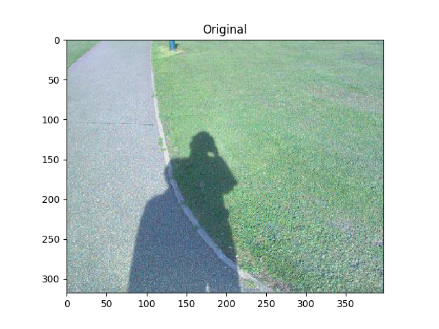
    img = cv2.imread(os.path.join(root, fl))
    img = cv2.cvtColor(img, cv2.COLOR_BGR2RGB)
    h, w = img.shape[:2]

    plt.imshow(img)
    plt.title('Original')
    plt.show()

    img = cv2.GaussianBlur(img, (5,5), 0)

    # Separate Channels
    r, g, b = cv2.split(img) 

    im_sum = np.sum(img, axis=2)
    im_mean = gmean(img, axis=2)

    # Create "normalized", mean, and rg chromaticity vectors
    #  We use mean (works better than norm). rg Chromaticity is
    #  for visualization
    n_r = np.ma.divide( 1.*r, g )
    n_b = np.ma.divide( 1.*b, g )

    mean_r = np.ma.divide(1.*r, im_mean)
    mean_g = np.ma.divide(1.*g, im_mean)
    mean_b = np.ma.divide(1.*b, im_mean)

    rg_chrom_r = np.ma.divide(1.*r, im_sum)
    rg_chrom_g = np.ma.divide(1.*g, im_sum)
    rg_chrom_b = np.ma.divide(1.*b, im_sum)

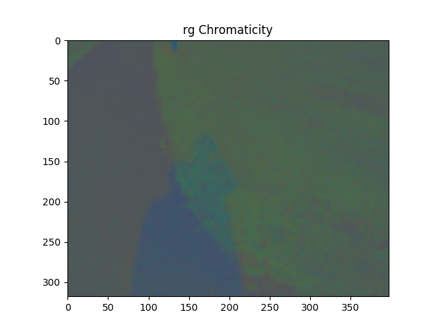
    # Visualize rg Chromaticity --> DEBUGGING
    rg_chrom = np.zeros_like(img)

    rg_chrom[:,:,0] = np.clip(np.uint8(rg_chrom_r*255), 0, 255)
    rg_chrom[:,:,1] = np.clip(np.uint8(rg_chrom_g*255), 0, 255)
    rg_chrom[:,:,2] = np.clip(np.uint8(rg_chrom_b*255), 0, 255)

    plt.imshow(rg_chrom)
    plt.title('rg Chromaticity')
    plt.show()

    #-----------------------
    ## 2. Take Logarithms ##
    #-----------------------

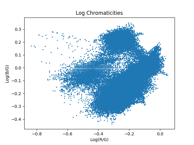
    l_rg = np.ma.log(n_r)
    l_bg = np.ma.log(n_b)

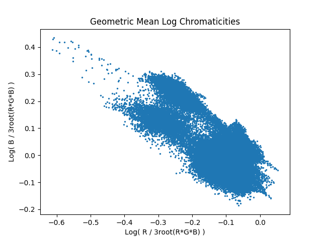
    log_r = np.ma.log(mean_r)
    log_g = np.ma.log(mean_g)
    log_b = np.ma.log(mean_b)

    ##  rho = np.zeros_like(img, dtype=np.float64)
    ##
    ##  rho[:,:,0] = log_r
    ##  rho[:,:,1] = log_g
    ##  rho[:,:,2] = log_b

    rho = cv2.merge((log_r, log_g, log_b))

    # Visualize Logarithms --> DEBUGGING
    plt.scatter(l_rg, l_bg, s = 2)
    plt.xlabel('Log(R/G)')
    plt.ylabel('Log(B/G)')
    plt.title('Log Chromaticities')
    plt.show()

    plt.scatter(log_r, log_b, s = 2)
    plt.xlabel('Log( R / 3root(R*G*B) )')
    plt.ylabel('Log( B / 3root(R*G*B) )')
    plt.title('Geometric Mean Log Chromaticities')
    plt.show()

    #----------------------------
    ## 3. Rotate through Theta ##
    #----------------------------
    u = 1./np.sqrt(3)*np.array([[1,1,1]]).T
    I = np.eye(3)

    tol = 1e-15

    P_u_norm = I - u.dot(u.T)
    U_, s, V_ = np.linalg.svd(P_u_norm, full_matrices = False)

    s[ np.where( s <= tol ) ] = 0.

    U = np.dot(np.eye(3)*np.sqrt(s), V_)
    U = U[ ~np.all( U == 0, axis = 1) ].T

    # Columns are upside down and column 2 is negated...?
    U = U[::-1,:]
    U[:,1] *= -1.

    ##  TRUE ARRAY:
    ##
    ##  U = np.array([[ 0.70710678,  0.40824829],
    ##                [-0.70710678,  0.40824829],
    ##                [ 0.        , -0.81649658]])

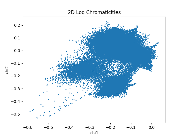
    chi = rho.dot(U) 

    # Visualize chi --> DEBUGGING
    plt.scatter(chi[:,:,0], chi[:,:,1], s = 2)
    plt.xlabel('chi1')
    plt.ylabel('chi2')
    plt.title('2D Log Chromaticities')
    plt.show()

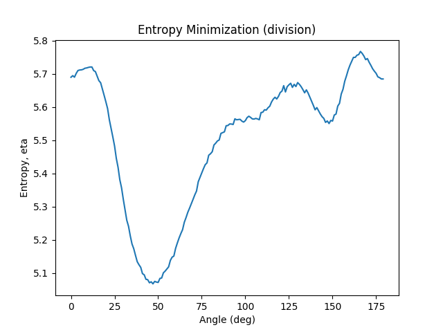
    e = np.array([[np.cos(np.radians(np.linspace(1, 180, 180))), \
                   np.sin(np.radians(np.linspace(1, 180, 180)))]])

    gs = chi.dot(e)

    prob = np.array([np.histogram(gs[...,i], bins='scott', density=True)[0] 
                      for i in range(np.size(gs, axis=3))])

    eta = np.array([entropy(p, base=2) for p in prob])

    plt.plot(eta)
    plt.xlabel('Angle (deg)')
    plt.ylabel('Entropy, eta')
    plt.title('Entropy Minimization')
    plt.show()

    theta_min = np.radians(np.argmin(eta))

    print('Min Angle: ', np.degrees(theta_min))

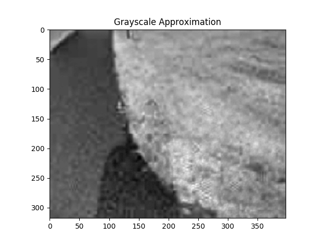
    e = np.array([[-1.*np.sin(theta_min)],
                  [np.cos(theta_min)]])

    gs_approx = chi.dot(e)

    # Visualize Grayscale Approximation --> DEBUGGING
    plt.imshow(gs_approx.squeeze(), cmap='gray')
    plt.title('Grayscale Approximation')
    plt.show()

    P_theta = np.ma.divide( np.dot(e, e.T), np.linalg.norm(e) )

    chi_theta = chi.dot(P_theta)
    rho_estim = chi_theta.dot(U.T)
    mean_estim = np.ma.exp(rho_estim)

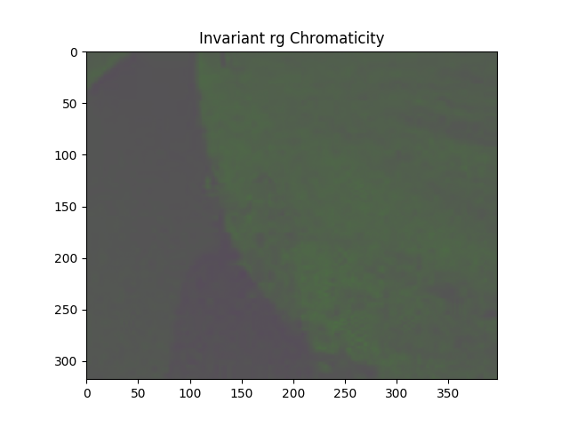
    estim = np.zeros_like(mean_estim, dtype=np.float64)

    estim[:,:,0] = np.divide(mean_estim[:,:,0], np.sum(mean_estim, axis=2))
    estim[:,:,1] = np.divide(mean_estim[:,:,1], np.sum(mean_estim, axis=2))
    estim[:,:,2] = np.divide(mean_estim[:,:,2], np.sum(mean_estim, axis=2))

    plt.imshow(estim)
    plt.title('Invariant rg Chromaticity')
    plt.show()

输出：