变时间步长卡尔曼滤波

Question

我有一些数据来表示从两个不同的传感器测量到的物体的位置。所以我需要做传感器融合。更困难的问题是，来自每个传感器的数据，基本上是在一个随机的时间到达。我想用pykalman来融合和平滑数据。pykalman如何处理可变时间戳数据？

数据的简化示例如下所示：

import pandas as pd
data={'time':\
['10:00:00.0','10:00:01.0','10:00:05.2','10:00:07.5','10:00:07.5','10:00:12.0','10:00:12.5']\
,'X':[10,10.1,20.2,25.0,25.1,35.1,35.0],'Y':[20,20.2,41,45,47,75.0,77.2],\
'Sensor':[1,2,1,1,2,1,2]}

df=pd.DataFrame(data,columns=['time','X','Y','Sensor'])
df.time=pd.to_datetime(df.time)
df=df.set_index('time')

这是：

df
Out[130]: 
                            X     Y  Sensor
time                                       
2017-12-01 10:00:00.000  10.0  20.0       1
2017-12-01 10:00:01.000  10.1  20.2       2
2017-12-01 10:00:05.200  20.2  41.0       1
2017-12-01 10:00:07.500  25.0  45.0       1
2017-12-01 10:00:07.500  25.1  47.0       2
2017-12-01 10:00:12.000  35.1  75.0       1
2017-12-01 10:00:12.500  35.0  77.2       2

对于传感器融合问题，我认为我可以重新塑造数据，这样我就有了位置X1，Y1，X2，Y2，而不仅仅是X，Y。(这是相关的：https://stackoverflow.com/questions/47386426/2-sensor-readings-fusion-yaw-pitch )

所以我的数据看起来是这样的：

df['X1']=df.X[df.Sensor==1]
df['Y1']=df.Y[df.Sensor==1]
df['X2']=df.X[df.Sensor==2]
df['Y2']=df.Y[df.Sensor==2]
df
Out[132]: 
                            X     Y  Sensor    X1    Y1    X2    Y2
time                                                               
2017-12-01 10:00:00.000  10.0  20.0       1  10.0  20.0   NaN   NaN
2017-12-01 10:00:01.000  10.1  20.2       2   NaN   NaN  10.1  20.2
2017-12-01 10:00:05.200  20.2  41.0       1  20.2  41.0   NaN   NaN
2017-12-01 10:00:07.500  25.0  45.0       1  25.0  45.0  25.1  47.0
2017-12-01 10:00:07.500  25.1  47.0       2  25.0  45.0  25.1  47.0
2017-12-01 10:00:12.000  35.1  75.0       1  35.1  75.0   NaN   NaN
2017-12-01 10:00:12.500  35.0  77.2       2   NaN   NaN  35.0  77.2

pykalman的文档表明它可以处理丢失的数据，但这是正确的吗？

但是，pykalman的文档对可变时间问题一点也不清楚。医生刚刚说：

卡尔曼滤波器和卡尔曼平滑器都可以使用随时间变化的参数。为了使用这一点，只需沿第一轴输入一个长的阵列n_timesteps：

>>> transition_offsets = [[-1], [0], [1], [2]]
>>> kf = KalmanFilter(transition_offsets=transition_offsets, n_dim_obs=1)

我还没有找到任何使用可变时间步骤的pykalman平滑器的例子。因此，任何使用我上述数据的指导、示例甚至示例都将是非常有用的。我不需要使用pykalman，但它似乎是平滑这些数据的有用工具。

*在@Anton下面添加的额外代码，我制作了一个使用光滑函数的有用代码的版本。奇怪的是，它似乎用同样的重量对待每一个观察，并让轨迹贯穿每一个观察。即使，如果我有一个很大的差异，传感器之间的方差值。我认为，在5.4,5.0点附近，过滤后的轨迹应该更接近传感器1点，因为这个点的方差较低。相反，轨迹正好指向每一个点，然后大转弯才能到达那里。

from pykalman import KalmanFilter
import numpy as np
import matplotlib.pyplot as plt

# reading data (quick and dirty)
Time=[]
RefX=[]
RefY=[]
Sensor=[]
X=[]
Y=[]

for line in open('data/dataset_01.csv'):
    f1, f2, f3, f4, f5, f6 = line.split(';')
    Time.append(float(f1))
    RefX.append(float(f2))
    RefY.append(float(f3))
    Sensor.append(float(f4))
    X.append(float(f5))
    Y.append(float(f6))

# Sensor 1 has a higher precision (max error = 0.1 m)
# Sensor 2 has a lower precision (max error = 0.3 m)

# Variance definition through 3-Sigma rule
Sensor_1_Variance = (0.1/3)**2;
Sensor_2_Variance = (0.3/3)**2;

# Filter Configuration

# time step
dt = Time[2] - Time[1]

# transition_matrix  
F = [[1,  0,  dt,   0], 
     [0,  1,   0,  dt],
     [0,  0,   1,   0],
     [0,  0,   0,   1]]   

# observation_matrix   
H = [[1, 0, 0, 0],
     [0, 1, 0, 0]]

# transition_covariance 
Q = [[1e-4,     0,     0,     0], 
     [   0,  1e-4,     0,     0],
     [   0,     0,  1e-4,     0],
     [   0,     0,     0,  1e-4]] 

# observation_covariance 
R_1 = [[Sensor_1_Variance, 0],
       [0, Sensor_1_Variance]]

R_2 = [[Sensor_2_Variance, 0],
       [0, Sensor_2_Variance]]

# initial_state_mean
X0 = [0,
      0,
      0,
      0]

# initial_state_covariance - assumed a bigger uncertainty in initial velocity
P0 = [[  0,    0,   0,   0], 
      [  0,    0,   0,   0],
      [  0,    0,   1,   0],
      [  0,    0,   0,   1]]

n_timesteps = len(Time)
n_dim_state = 4
filtered_state_means = np.zeros((n_timesteps, n_dim_state))
filtered_state_covariances = np.zeros((n_timesteps, n_dim_state, n_dim_state))

import numpy.ma as ma

obs_cov=np.zeros([n_timesteps,2,2])
obs=np.zeros([n_timesteps,2])

for t in range(n_timesteps):
    if Sensor[t] == 0:
        obs[t]=None
    else:
        obs[t] = [X[t], Y[t]]
        if Sensor[t] == 1:
            obs_cov[t] = np.asarray(R_1)
        else:
            obs_cov[t] = np.asarray(R_2)

ma_obs=ma.masked_invalid(obs)

ma_obs_cov=ma.masked_invalid(obs_cov)

# Kalman-Filter initialization
kf = KalmanFilter(transition_matrices = F, 
                  observation_matrices = H, 
                  transition_covariance = Q, 
                  observation_covariance = ma_obs_cov, # the covariance will be adapted depending on Sensor_ID
                  initial_state_mean = X0, 
                  initial_state_covariance = P0)

filtered_state_means, filtered_state_covariances=kf.smooth(ma_obs)


# extracting the Sensor update points for the plot        
Sensor_1_update_index = [i for i, x in enumerate(Sensor) if x == 1]    
Sensor_2_update_index = [i for i, x in enumerate(Sensor) if x == 2]     

Sensor_1_update_X = [ X[i] for i in Sensor_1_update_index ]        
Sensor_1_update_Y = [ Y[i] for i in Sensor_1_update_index ]   

Sensor_2_update_X = [ X[i] for i in Sensor_2_update_index ]        
Sensor_2_update_Y = [ Y[i] for i in Sensor_2_update_index ] 

# plot of the resulted trajectory
plt.plot(RefX, RefY, "k-", label="Real Trajectory")
plt.plot(Sensor_1_update_X, Sensor_1_update_Y, "ro", label="Sensor 1")
plt.plot(Sensor_2_update_X, Sensor_2_update_Y, "bo", label="Sensor 2")
plt.plot(filtered_state_means[:, 0], filtered_state_means[:, 1], "g.", label="Filtered Trajectory", markersize=1)
plt.grid()
plt.legend(loc="upper left")
plt.show()    

Answer 1

对于卡尔曼滤波器来说，用固定的时间步长表示输入数据是非常有用的。您的传感器随机发送数据，因此您可以为您的系统定义最小的重要时间步骤，并使用此步骤对时间轴进行离散化。

例如，一个传感器大约每0.2秒发送一次数据，第二个传感器每0.5秒发送一次数据。因此，最小的时间步长可能是0.01秒(在这里，您需要在计算时间和所需的精度之间找到一个折衷)。

您的数据如下所示：

Time    Sensor  X       Y
0,52        0   0       0
0,53        1   0,3417  0,2988
0,54        0   0       0
0,56        0   0       0
0,57        0   0       0
0,55        0   0       0
0,58        0   0       0
0,59        2   0,4247  0,3779
0,60        0   0       0
0,61        0   0       0
0,62        0   0       0

现在，您需要根据您的观察结果调用Pykalman函数filter_update。如果没有观察，过滤器将根据前一个状态预测下一个状态。如果有一个观察，它纠正系统的状态。

也许你的传感器有不同的精确度。因此，您可以根据传感器的方差指定观测协方差。

为了证明这一想法，我生成了一个二维轨迹，并随机放置了两个传感器的测量，具有不同的精度。

Sensor1: mean update time = 1.0s; max error = 0.1m;
Sensor2: mean update time = 0.7s; max error = 0.3m;

结果如下：

​

​

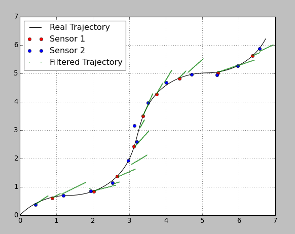
我故意选择了非常糟糕的参数，所以我们可以看到预测和修正的步骤。在传感器更新之间，滤波器根据前一步的恒定速度预测轨迹。一旦更新，过滤器就会根据传感器的变化来校正位置。第二传感器的精度很差，影响了系统的重量。

下面是我的python代码：

from pykalman import KalmanFilter
import numpy as np
import matplotlib.pyplot as plt

# reading data (quick and dirty)
Time=[]
RefX=[]
RefY=[]
Sensor=[]
X=[]
Y=[]

for line in open('data/dataset_01.csv'):
    f1, f2, f3, f4, f5, f6 = line.split(';')
    Time.append(float(f1))
    RefX.append(float(f2))
    RefY.append(float(f3))
    Sensor.append(float(f4))
    X.append(float(f5))
    Y.append(float(f6))

# Sensor 1 has a higher precision (max error = 0.1 m)
# Sensor 2 has a lower precision (max error = 0.3 m)

# Variance definition through 3-Sigma rule
Sensor_1_Variance = (0.1/3)**2;
Sensor_2_Variance = (0.3/3)**2;

# Filter Configuration

# time step
dt = Time[2] - Time[1]

# transition_matrix  
F = [[1,  0,  dt,   0], 
     [0,  1,   0,  dt],
     [0,  0,   1,   0],
     [0,  0,   0,   1]]   

# observation_matrix   
H = [[1, 0, 0, 0],
     [0, 1, 0, 0]]

# transition_covariance 
Q = [[1e-4,     0,     0,     0], 
     [   0,  1e-4,     0,     0],
     [   0,     0,  1e-4,     0],
     [   0,     0,     0,  1e-4]] 

# observation_covariance 
R_1 = [[Sensor_1_Variance, 0],
       [0, Sensor_1_Variance]]

R_2 = [[Sensor_2_Variance, 0],
       [0, Sensor_2_Variance]]

# initial_state_mean
X0 = [0,
      0,
      0,
      0]

# initial_state_covariance - assumed a bigger uncertainty in initial velocity
P0 = [[  0,    0,   0,   0], 
      [  0,    0,   0,   0],
      [  0,    0,   1,   0],
      [  0,    0,   0,   1]]

n_timesteps = len(Time)
n_dim_state = 4
filtered_state_means = np.zeros((n_timesteps, n_dim_state))
filtered_state_covariances = np.zeros((n_timesteps, n_dim_state, n_dim_state))

# Kalman-Filter initialization
kf = KalmanFilter(transition_matrices = F, 
                  observation_matrices = H, 
                  transition_covariance = Q, 
                  observation_covariance = R_1, # the covariance will be adapted depending on Sensor_ID
                  initial_state_mean = X0, 
                  initial_state_covariance = P0)


# iterative estimation for each new measurement
for t in range(n_timesteps):
    if t == 0:
        filtered_state_means[t] = X0
        filtered_state_covariances[t] = P0
    else:

        # the observation and its covariance have to be switched depending on Sensor_Id 
        #     Sensor_ID == 0: no observation
        #     Sensor_ID == 1: Sensor 1
        #     Sensor_ID == 2: Sensor 2

        if Sensor[t] == 0:
            obs = None
            obs_cov = None
        else:
            obs = [X[t], Y[t]]

            if Sensor[t] == 1:
                obs_cov = np.asarray(R_1)
            else:
                obs_cov = np.asarray(R_2)

        filtered_state_means[t], filtered_state_covariances[t] = (
        kf.filter_update(
            filtered_state_means[t-1],
            filtered_state_covariances[t-1],
            observation = obs,
            observation_covariance = obs_cov)
        )

# extracting the Sensor update points for the plot        
Sensor_1_update_index = [i for i, x in enumerate(Sensor) if x == 1]    
Sensor_2_update_index = [i for i, x in enumerate(Sensor) if x == 2]     

Sensor_1_update_X = [ X[i] for i in Sensor_1_update_index ]        
Sensor_1_update_Y = [ Y[i] for i in Sensor_1_update_index ]   

Sensor_2_update_X = [ X[i] for i in Sensor_2_update_index ]        
Sensor_2_update_Y = [ Y[i] for i in Sensor_2_update_index ] 

# plot of the resulted trajectory
plt.plot(RefX, RefY, "k-", label="Real Trajectory")
plt.plot(Sensor_1_update_X, Sensor_1_update_Y, "ro", label="Sensor 1")
plt.plot(Sensor_2_update_X, Sensor_2_update_Y, "bo", label="Sensor 2")
plt.plot(filtered_state_means[:, 0], filtered_state_means[:, 1], "g.", label="Filtered Trajectory", markersize=1)
plt.grid()
plt.legend(loc="upper left")
plt.show()    

我把csv文件放在这里上，这样您就可以执行代码了。

我希望我能帮你。

更新

关于变量转移矩阵的建议的一些信息。我想说，这取决于你的传感器的可用性和对评估结果的要求。

在这里，我用一个常数和一个可变的过渡矩阵绘制了相同的估计(我改变了过渡协方差矩阵，否则估计太糟糕了，因为滤波器的“刚度”很高)：

​

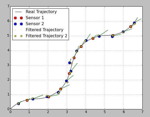
正如你所看到的，黄色标记的估计位置是相当好的。但是！传感器读数之间没有任何信息。使用变量转移矩阵可以避免在读数之间的预测步骤，并且不知道系统发生了什么。如果你的阅读率很高的话，它就足够好了，但除此之外，它可能是一个不利因素。

以下是更新的代码：

from pykalman import KalmanFilter
import numpy as np
import matplotlib.pyplot as plt

# reading data (quick and dirty)
Time=[]
RefX=[]
RefY=[]
Sensor=[]
X=[]
Y=[]

for line in open('data/dataset_01.csv'):
    f1, f2, f3, f4, f5, f6 = line.split(';')
    Time.append(float(f1))
    RefX.append(float(f2))
    RefY.append(float(f3))
    Sensor.append(float(f4))
    X.append(float(f5))
    Y.append(float(f6))

# Sensor 1 has a higher precision (max error = 0.1 m)
# Sensor 2 has a lower precision (max error = 0.3 m)

# Variance definition through 3-Sigma rule
Sensor_1_Variance = (0.1/3)**2;
Sensor_2_Variance = (0.3/3)**2;

# Filter Configuration

# time step
dt = Time[2] - Time[1]

# transition_matrix  
F = [[1,  0,  dt,   0], 
     [0,  1,   0,  dt],
     [0,  0,   1,   0],
     [0,  0,   0,   1]]   

# observation_matrix   
H = [[1, 0, 0, 0],
     [0, 1, 0, 0]]

# transition_covariance 
Q = [[1e-2,     0,     0,     0], 
     [   0,  1e-2,     0,     0],
     [   0,     0,  1e-2,     0],
     [   0,     0,     0,  1e-2]] 

# observation_covariance 
R_1 = [[Sensor_1_Variance, 0],
       [0, Sensor_1_Variance]]

R_2 = [[Sensor_2_Variance, 0],
       [0, Sensor_2_Variance]]

# initial_state_mean
X0 = [0,
      0,
      0,
      0]

# initial_state_covariance - assumed a bigger uncertainty in initial velocity
P0 = [[  0,    0,   0,   0], 
      [  0,    0,   0,   0],
      [  0,    0,   1,   0],
      [  0,    0,   0,   1]]

n_timesteps = len(Time)
n_dim_state = 4

filtered_state_means = np.zeros((n_timesteps, n_dim_state))
filtered_state_covariances = np.zeros((n_timesteps, n_dim_state, n_dim_state))

filtered_state_means2 = np.zeros((n_timesteps, n_dim_state))
filtered_state_covariances2 = np.zeros((n_timesteps, n_dim_state, n_dim_state))

# Kalman-Filter initialization
kf = KalmanFilter(transition_matrices = F, 
                  observation_matrices = H, 
                  transition_covariance = Q, 
                  observation_covariance = R_1, # the covariance will be adapted depending on Sensor_ID
                  initial_state_mean = X0, 
                  initial_state_covariance = P0)

# Kalman-Filter initialization (Different F Matrices depending on DT)
kf2 = KalmanFilter(transition_matrices = F, 
                  observation_matrices = H, 
                  transition_covariance = Q, 
                  observation_covariance = R_1, # the covariance will be adapted depending on Sensor_ID
                  initial_state_mean = X0, 
                  initial_state_covariance = P0)


# iterative estimation for each new measurement
for t in range(n_timesteps):
    if t == 0:
        filtered_state_means[t] = X0
        filtered_state_covariances[t] = P0

        # For second filter
        filtered_state_means2[t] = X0
        filtered_state_covariances2[t] = P0

        timestamp = Time[t]
        old_t = t
    else:

        # the observation and its covariance have to be switched depending on Sensor_Id 
        #     Sensor_ID == 0: no observation
        #     Sensor_ID == 1: Sensor 1
        #     Sensor_ID == 2: Sensor 2

        if Sensor[t] == 0:
            obs = None
            obs_cov = None
        else:
            obs = [X[t], Y[t]]

            if Sensor[t] == 1:
                obs_cov = np.asarray(R_1)
            else:
                obs_cov = np.asarray(R_2)

        filtered_state_means[t], filtered_state_covariances[t] = (
        kf.filter_update(
            filtered_state_means[t-1],
            filtered_state_covariances[t-1],
            observation = obs,
            observation_covariance = obs_cov)
        )

        #For the second filter
        if Sensor[t] != 0:

            obs2 = [X[t], Y[t]]

            if Sensor[t] == 1:
                obs_cov2 = np.asarray(R_1)
            else:
                obs_cov2 = np.asarray(R_2)  

            dt2 = Time[t] - timestamp

            timestamp = Time[t]        

            # transition_matrix  
            F2 = [[1,  0,  dt2,    0], 
                  [0,  1,    0,  dt2],
                  [0,  0,    1,    0],
                  [0,  0,    0,    1]] 

            filtered_state_means2[t], filtered_state_covariances2[t] = (
            kf2.filter_update(
                filtered_state_means2[old_t],
                filtered_state_covariances2[old_t],
                observation = obs2,
                observation_covariance = obs_cov2,
                transition_matrix = np.asarray(F2))
            )      

            old_t = t

# extracting the Sensor update points for the plot        
Sensor_1_update_index = [i for i, x in enumerate(Sensor) if x == 1]    
Sensor_2_update_index = [i for i, x in enumerate(Sensor) if x == 2]     

Sensor_1_update_X = [ X[i] for i in Sensor_1_update_index ]        
Sensor_1_update_Y = [ Y[i] for i in Sensor_1_update_index ]   

Sensor_2_update_X = [ X[i] for i in Sensor_2_update_index ]        
Sensor_2_update_Y = [ Y[i] for i in Sensor_2_update_index ] 

# plot of the resulted trajectory
plt.plot(RefX, RefY, "k-", label="Real Trajectory")
plt.plot(Sensor_1_update_X, Sensor_1_update_Y, "ro", label="Sensor 1", markersize=9)
plt.plot(Sensor_2_update_X, Sensor_2_update_Y, "bo", label="Sensor 2", markersize=9)
plt.plot(filtered_state_means[:, 0], filtered_state_means[:, 1], "g.", label="Filtered Trajectory", markersize=1)
plt.plot(filtered_state_means2[:, 0], filtered_state_means2[:, 1], "yo", label="Filtered Trajectory 2", markersize=6)
plt.grid()
plt.legend(loc="upper left")
plt.show()    

我在这段代码中没有实现的另一个要点是:在使用变量转换矩阵时，还需要改变转换协方差矩阵(取决于当前的dt)。

这是个有趣的话题。让我知道什么样的估计最适合你的问题。