ggMarginal忽略choord_cartesian。如何改变边缘尺度？

Question

我试着用‘m图绘制2D密度图，并添加边缘直方图。问题是多边形呈现是愚蠢的，需要额外的填充来呈现超出轴限制的值(例如，在这种情况下，我将限制设置在0到1之间，因为超出这个范围的值没有物理意义)。我仍然需要密度估计，因为它通常比块状二维热图要干净得多。

除了彻底废除ggMarginal并花费50行代码试图对直方图之外，还有解决这个问题的方法吗？

难看的线条：

​

​

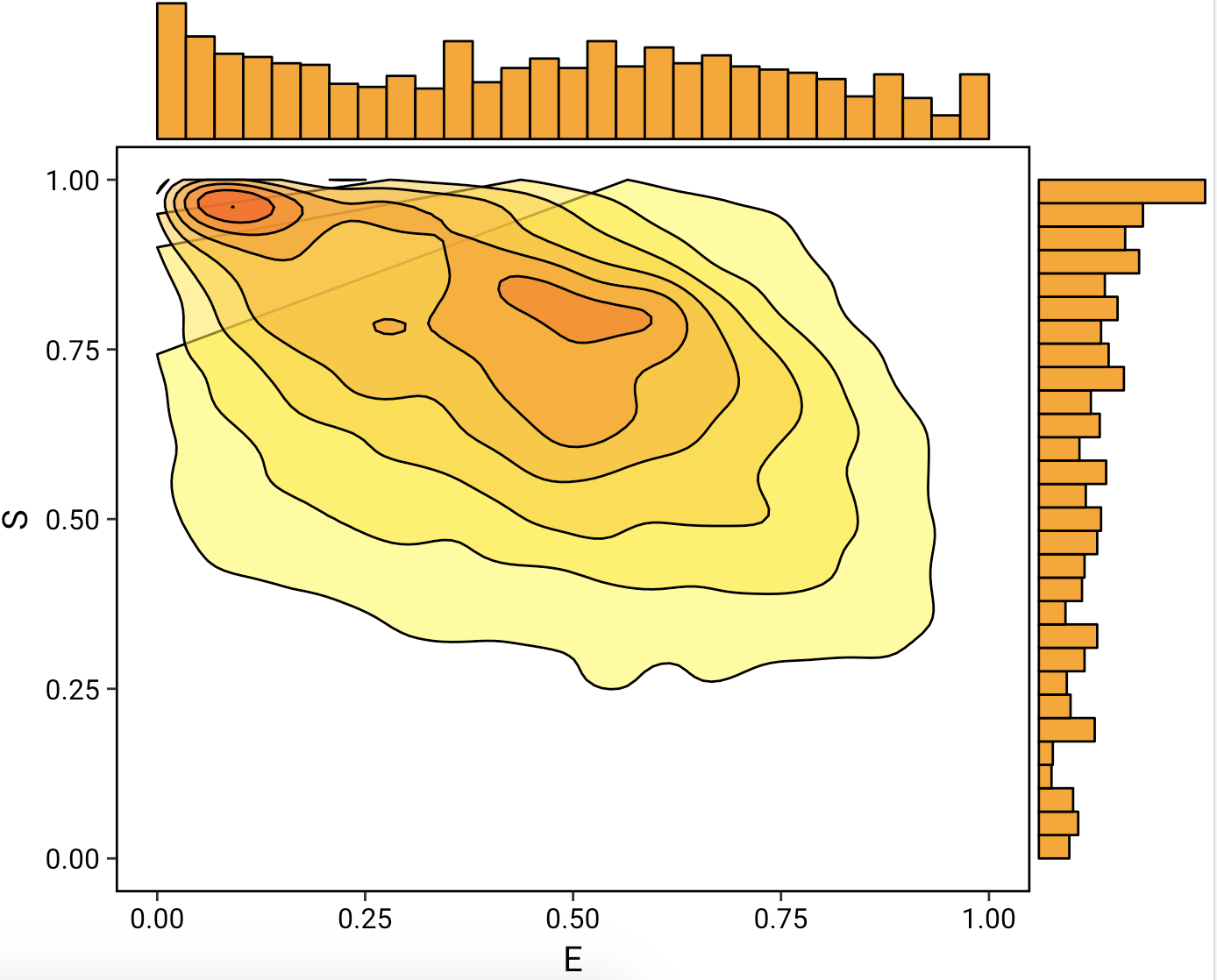
choord_cartesian()**，现在正在渲染作品，但是ggMarginal忽略了，它摧毁了情节：**

​

这里的数据：http://pasted.co/b581605a

dataset <- read.csv("~/Desktop/dataset.csv")

library(ggplot2)
library(ggthemes)
library(ggExtra)
plot_center <- ggplot(data = dataset, aes(x = E,
                                          y = S)) +
    stat_density2d(aes(fill=..level..),
                   bins= 8, 
                   geom="polygon",
                   col = "black",
                   alpha = 0.5) + 
    scale_fill_continuous(low = "yellow",
                          high = "red") +
    scale_x_continuous(limits = c(-1,2)) + # Render padding for polygon
    scale_y_continuous(limits = c(-1,2)) + #
    coord_cartesian(ylim = c(0, 1),
                    xlim = c(0, 1)) +
    theme_tufte(base_size = 15, base_family = "Roboto") +
    theme(axis.text    = element_text(color = "black"),
          panel.border = element_rect(colour = "black", fill=NA, size=1),
          legend.text  = element_text(size = 12, family = "Roboto"),
          legend.title = element_blank(),
          legend.position = "none")

ggMarginal(plot_center,
           type = "histogram",
           col = "black",
           fill = "orange",
           margins = "both")

Answer 1

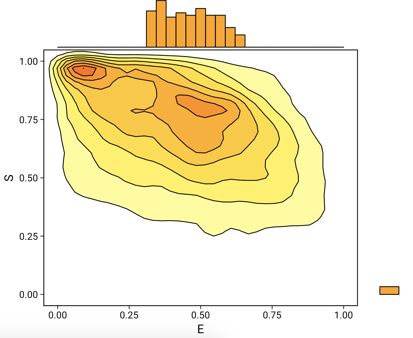
您可以使用xlim()和ylim()而不是coord_cartesian来解决这个问题。

dataset <- read.csv("~/Desktop/dataset.csv")

library(ggplot2)
library(ggthemes)
library(ggExtra)

plot_center <- ggplot(data = dataset, aes(x = E,
                                          y = S)) +
    stat_density2d(aes(fill=..level..),
                   bins= 8, 
                   geom="polygon",
                   col = "black",
                   alpha = 0.5) + 
    scale_fill_continuous(low = "yellow",
                          high = "red") +
    scale_x_continuous(limits = c(-1,2)) + # Render padding for polygon
    scale_y_continuous(limits = c(-1,2)) + #
    xlim(c(0,1)) +
    ylim(c(0,1)) +
    theme_tufte(base_size = 15, base_family = "Roboto") +
    theme(axis.text    = element_text(color = "black"),
          panel.border = element_rect(colour = "black", fill=NA, size=1),
          legend.text  = element_text(size = 12, family = "Roboto"),
          legend.title = element_blank(),
          legend.position = "none")

ggMarginal(plot_center,
           type = "histogram",
           col = "black",
           fill = "orange",
           margins = "both")