用公式计算反三角函数

Question

我一直试图创建计算三角函数的自定义计算器。除了Chebyshev幽门分类法和/或Cordic算法外，我还使用了泰勒级数，它在小数点的几个位都是精确的。

这是我为计算不需要任何模块的简单三角函数而创建的：

from __future__ import division

def sqrt(n):
  ans = n ** 0.5
  return ans

def factorial(n):
  k = 1
  for i in range(1, n+1):
    k = i * k

  return k 

def sin(d):
  pi = 3.14159265359
  n = 180 / int(d) # 180 degrees = pi radians
  x = pi / n # Converting degrees to radians
  ans = x - ( x ** 3 / factorial(3) ) + ( x ** 5 / factorial(5) ) - ( x ** 7 / factorial(7) ) + ( x ** 9 / factorial(9) )
  return ans 

def cos(d):
  pi = 3.14159265359
  n = 180 / int(d) 
  x = pi / n 
  ans = 1 - ( x ** 2 / factorial(2) ) + ( x ** 4 / factorial(4) ) - ( x ** 6 / factorial(6) ) + ( x ** 8 / factorial(8) )
  return ans 

def tan(d): 
  ans = sin(d) / sqrt(1 - sin(d) ** 2)
  return ans 

不幸的是，我找不到任何可以帮助我解释Python的反三角函数公式的来源。我还试着将罪恶(X)置于-1 (sin(x) ** -1)的能力中，但它并没有像预期的那样起作用。

在Python中，什么是最好的解决方案(在最好的情况下，我指的是与Taylor级数一样精确的最简单的方法)？这是可能的幂级数，还是我需要使用cordic算法？

Answer 1

这个问题的范围很广，但是这里有一些简单的想法(和代码！)这可能是计算arctan的起点。首先是好的老泰勒系列。为了简单起见，我们使用了固定数量的术语；在实践中，您可能希望根据x的大小动态确定要使用的术语数量，或者引入某种收敛准则。在一定数量的条件下，我们可以使用类似于Horner方案的方法来有效地进行评估。

def arctan_taylor(x, terms=9):
    """
    Compute arctan for small x via Taylor polynomials.

    Uses a fixed number of terms. The default of 9 should give good results for
    abs(x) < 0.1. Results will become poorer as abs(x) increases, becoming
    unusable as abs(x) approaches 1.0 (the radius of convergence of the
    series).
    """
    # Uses Horner's method for evaluation.
    t = 0.0
    for n in range(2*terms-1, 0, -2):
        t = 1.0/n - x*x*t
    return x * t

上面的代码对于小x (比如绝对值小于0.1 )提供了很好的结果，但是随着x的增大，精度下降了，对于abs(x) > 1.0，不管我们抛出了多少项(或额外的精度)，这个系列都不会收敛。因此，我们需要一种更好的方法来计算较大的x。一种解决方案是通过标识arctan(x) = 2 * arctan(x / (1 + sqrt(1 + x^2)))使用参数约简。这给出了以下代码，它构建在arctan_taylor之上，为广泛的x提供了合理的结果(但是在计算x*x时要小心可能的溢出和下溢)。

import math

def arctan_taylor_with_reduction(x, terms=9, threshold=0.1):
    """
    Compute arctan via argument reduction and Taylor series.

    Applies reduction steps until x is below `threshold`,
    then uses Taylor series.
    """
    reductions = 0
    while abs(x) > threshold:
        x = x / (1 + math.sqrt(1 + x*x))
        reductions += 1

    return arctan_taylor(x, terms=terms) * 2**reductions

或者，给定tan的现有实现，您可以使用传统的根查找方法简单地找到方程tan(y) = x的解决方案y。由于arctan自然存在于区间(-pi/2, pi/2)中，所以二分法搜索效果很好：

def arctan_from_tan(x, tolerance=1e-15):
    """
    Compute arctan as the inverse of tan, via bisection search. This assumes
    that you already have a high quality tan function.
    """
    low, high = -0.5 * math.pi, 0.5 * math.pi
    while high - low > tolerance:
        mid = 0.5 * (low + high)
        if math.tan(mid) < x:
            low = mid
        else:
            high = mid
    return 0.5 * (low + high)

最后，为了好玩，这里有一个类似CORDIC的实现，它实际上更适合于低级别的实现，而不是Python。这里的想法是，一劳永逸地预先计算1、1/2, 1/4,等的arctan值表，然后使用这些表计算一般的arctan值，实质上是通过计算对真实角度的逐次逼近。值得注意的是，在计算前的一步之后，arctan计算只需要以2的幂进行加、减和乘。(当然，在Python级别上，这些乘法并不比任何其他乘法更有效，但更接近硬件，这可能会产生很大的差异。)

cordic_table_size = 60
cordic_table = [(2**-i, math.atan(2**-i))
                 for i in range(cordic_table_size)]

def arctan_cordic(y, x=1.0):
    """
    Compute arctan(y/x), assuming x positive, via CORDIC-like method.
    """
    r = 0.0
    for t, a in cordic_table:
        if y < 0:
            r, x, y = r - a, x - t*y, y + t*x
        else:
            r, x, y = r + a, x + t*y, y - t*x
    return r

上述每一种方法都有其优点和缺点，所有上述代码都可以通过多种方式加以改进。我鼓励你去尝试和探索。

综上所述，下面是对少量未仔细选择的测试值调用上述函数的结果，并与标准库math.atan函数的输出进行比较：

test_values = [2.314, 0.0123, -0.56, 168.9]
for value in test_values:
    print("{:20.15g} {:20.15g} {:20.15g} {:20.15g}".format(
        math.atan(value),
        arctan_taylor_with_reduction(value),
        arctan_from_tan(value),
        arctan_cordic(value),
    ))

我的机器上的输出：

    1.16288340166519     1.16288340166519     1.16288340166519     1.16288340166519
     0.0122993797673      0.0122993797673   0.0122993797673002   0.0122993797672999
  -0.510488321916776   -0.510488321916776   -0.510488321916776   -0.510488321916776
    1.56487573286064     1.56487573286064     1.56487573286064     1.56487573286064

Answer 2

做任何逆函数的最简单的方法是使用二进制搜索。

1. 定义 设函数 X= g(y) 我们要对它的逆序进行编码： Y= f(x) = f(g(y)) x= y=
2. 浮标bin搜索 您可以通过整数运算来访问尾数位，如下所示：

- [Any Faster RMS Value Calculation in C?](https://stackoverflow.com/a/28808095/2521214)

但是，如果在计算之前不知道结果的指数，那么也需要使用floats搜索。

因此，二进制搜索背后的想法是将y的尾数从y1一点一点地转换为y0，从MSB到LSB。然后调用直接函数g(y)，如果结果交叉x，则恢复最后一位更改。

在使用浮点数的情况下，可以使用保持尾数位的近似值的变量，而不是整数位访问。这将消除未知指数问题。因此，在开始时，将y = y0和实际位设置为、MSB、值和b=(y1-y0)/2。在每次迭代之后，将其减半，并进行尽可能多的迭代，如获得尾数位n.通过这种方式，可以在n精度范围内获得(y1-y0)/2^n迭代的结果。

如果你的反函数不是单调的，把它分解成单调的间隔，然后把每一个处理成单独的二进制搜索。

函数的增减决定了交叉条件的方向(使用<或>)。

C++ acos示例

​

​

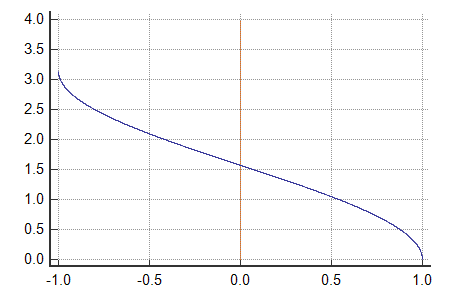
因此，y = acos(x)是在x = <-1,+1> , y = <0,M_PI>上定义的，递减是这样的：

double f64_acos(double x)
    {
    const int n=52;         // mantisa bits
    double y,y0,b;
    int i;
    // handle domain error
    if (x<-1.0) return 0;
    if (x>+1.0) return 0;
    // x = <-1,+1> , y = <0,M_PI> , decreasing
    for (y= 0.0,b=0.5*M_PI,i=0;i<n;i++,b*=0.5)  // y is min, b is half of max and halving each iteration
        {
        y0=y;                   // remember original y
        y+=b;                   // try set "bit"
        if (cos(y)<x) y=y0;     // if result cross x return to original y decreasing is <  and increasing is >
        }
    return y;
    }

我是这样测试的：

double x0,x1,y;
for (x0=0.0;x0<M_PI;x0+=M_PI*0.01)  // cycle all angle range <0,M_PI>
    {
    y=cos(x0);              // direct function (from math.h)
    x1=f64_acos(y);         // my inverse function
    if (fabs(x1-x0)>1e-9)   // check result and output to log if error
     Form1->mm_log->Lines->Add(AnsiString().sprintf("acos(%8.3lf) = %8.3lf != %8.3lf",y,x0,x1));
    }

没有发现任何区别..。因此，实现是正确的工作。对于52位尾数的粗二进制搜索，通常比多项式逼近慢。另一方面，实现是如此简单.

Notes

如果你不想处理单调的间隔，你可以试试。

• approximation search

在处理角度测量函数时，您需要处理奇点，以避免NaN或除以零等。

如果您感兴趣，这里有更多bin搜索示例(主要是关于整数)。

• Power by squaring for negative exponents it contains