Python中的自相关代码产生错误(吉他音高检测)

Question

这个链接为基于自相关的基音检测算法提供了代码.我用它来探测简单吉他旋律中的音高。

总的来说，它产生了很好的效果。例如，对于旋律C4、C#4、D4、D#4、E4，它输出：

262.743653536
272.144441273
290.826273006
310.431336809
327.094621169

这与正确的音符有关。

但是，在某些情况下，如这音频文件(E4、F4、F#4、G4、G#4、A4、A#4、B4)，它会产生错误：

325.861452246
13381.6439242
367.518651703
391.479384923
414.604661221
218.345286173
466.503751322
244.994090035

更具体地说，这里有三个错误：13381 B4 代替F4 (~350 B4)(奇怪的误差)，还有218 B4代替A4 (440 B4)和244 B4代替B4(~493 B4)，后者是倍频程误差。

我想这两个错误是由不同的东西引起的吧？以下是代码：

slices = segment_signal(y, sr)
for segment in slices:
  pitch = freq_from_autocorr(segment, sr)
  print pitch

def segment_signal(y, sr, onset_frames=None, offset=0.1):
  if (onset_frames == None):
    onset_frames = remove_dense_onsets(librosa.onset.onset_detect(y=y, sr=sr))

  offset_samples = int(librosa.time_to_samples(offset, sr))

  print onset_frames

  slices = np.array([y[i : i + offset_samples] for i
    in librosa.frames_to_samples(onset_frames)])

  return slices

您可以在上面的第一个链接中看到freq_from_autocorr函数。

我唯一认为我改变的是这句话：

corr = corr[len(corr)/2:]

我已将其替换为：

corr = corr[int(len(corr)/2):]

更新

我注意到我使用的offset最小(用于检测每个音高的信号段越小)，我得到的高频(10000+ Hz)误差越大。

特别是，我注意到在这些情况下不同的部分(10000+ Hz)是i_peak值的计算。在没有错误的情况下，它是在50-150的范围内，在错误的情况下是3-5。

Answer 1

您所链接的代码片段中的自相关函数并不特别健壮。为了得到正确的结果，需要在自相关曲线的左手侧定位第一个峰值。其他开发人员使用的方法(调用numpy.argmax()函数)并不总是找到正确的值。

我使用桃子包实现了一个稍微健壮的版本。我也不保证它是完全健壮的，但无论如何，它比您以前使用的freq_from_autocorr()函数的版本获得了更好的结果。

下面列出了我的示例解决方案：

import librosa
import numpy as np
import matplotlib.pyplot as plt
from scipy.signal import fftconvolve
from pprint import pprint
import peakutils

def freq_from_autocorr(signal, fs):
    # Calculate autocorrelation (same thing as convolution, but with one input
    # reversed in time), and throw away the negative lags
    signal -= np.mean(signal)  # Remove DC offset
    corr = fftconvolve(signal, signal[::-1], mode='full')
    corr = corr[len(corr)//2:]

    # Find the first peak on the left
    i_peak = peakutils.indexes(corr, thres=0.8, min_dist=5)[0]
    i_interp = parabolic(corr, i_peak)[0]

    return fs / i_interp, corr, i_interp

def parabolic(f, x):
    """
    Quadratic interpolation for estimating the true position of an
    inter-sample maximum when nearby samples are known.

    f is a vector and x is an index for that vector.

    Returns (vx, vy), the coordinates of the vertex of a parabola that goes
    through point x and its two neighbors.

    Example:
    Defining a vector f with a local maximum at index 3 (= 6), find local
    maximum if points 2, 3, and 4 actually defined a parabola.

    In [3]: f = [2, 3, 1, 6, 4, 2, 3, 1]

    In [4]: parabolic(f, argmax(f))
    Out[4]: (3.2142857142857144, 6.1607142857142856)
    """
    xv = 1/2. * (f[x-1] - f[x+1]) / (f[x-1] - 2 * f[x] + f[x+1]) + x
    yv = f[x] - 1/4. * (f[x-1] - f[x+1]) * (xv - x)
    return (xv, yv)

# Time window after initial onset (in units of seconds)
window = 0.1

# Open the file and obtain the sampling rate
y, sr = librosa.core.load("./Vocaroo_s1A26VqpKgT0.mp3")
idx = np.arange(len(y))

# Set the window size in terms of number of samples
winsamp = int(window * sr)

# Calcualte the onset frames in the usual way
onset_frames = librosa.onset.onset_detect(y=y, sr=sr)
onstm = librosa.frames_to_time(onset_frames, sr=sr)

fqlist = [] # List of estimated frequencies, one per note
crlist = [] # List of autocorrelation arrays, one array per note
iplist = [] # List of peak interpolated peak indices, one per note
for tm in onstm:
    startidx = int(tm * sr)
    freq, corr, ip = freq_from_autocorr(y[startidx:startidx+winsamp], sr)
    fqlist.append(freq)
    crlist.append(corr)
    iplist.append(ip)    

pprint(fqlist)

# Choose which notes to plot (it's set to show all 8 notes in this case)
plidx = [0, 1, 2, 3, 4, 5, 6, 7]

# Plot amplitude curves of all notes in the plidx list 
fgwin = plt.figure(figsize=[8, 10])
fgwin.subplots_adjust(bottom=0.0, top=0.98, hspace=0.3)
axwin = []
ii = 1
for tm in onstm[plidx]:
    axwin.append(fgwin.add_subplot(len(plidx)+1, 1, ii))
    startidx = int(tm * sr)
    axwin[-1].plot(np.arange(startidx, startidx+winsamp), y[startidx:startidx+winsamp])
    ii += 1
axwin[-1].set_xlabel('Sample ID Number', fontsize=18)
fgwin.show()

# Plot autocorrelation function of all notes in the plidx list
fgcorr = plt.figure(figsize=[8,10])
fgcorr.subplots_adjust(bottom=0.0, top=0.98, hspace=0.3)
axcorr = []
ii = 1
for cr, ip in zip([crlist[ii] for ii in plidx], [iplist[ij] for ij in plidx]):
    if ii == 1:
        shax = None
    else:
        shax = axcorr[0]
    axcorr.append(fgcorr.add_subplot(len(plidx)+1, 1, ii, sharex=shax))
    axcorr[-1].plot(np.arange(500), cr[0:500])
    # Plot the location of the leftmost peak
    axcorr[-1].axvline(ip, color='r')
    ii += 1
axcorr[-1].set_xlabel('Time Lag Index (Zoomed)', fontsize=18)
fgcorr.show()

打印的输出结果如下：

In [1]: %run autocorr.py
[325.81996740236065,
 346.43374761017725,
 367.12435233192753,
 390.17291696559079,
 412.9358117076161,
 436.04054933498134,
 465.38986619237039,
 490.34120132405866]

我的代码样本生成的第一个数字描述了在每次检测到的起始时间之后接下来的0.1秒的幅度曲线：

​

​

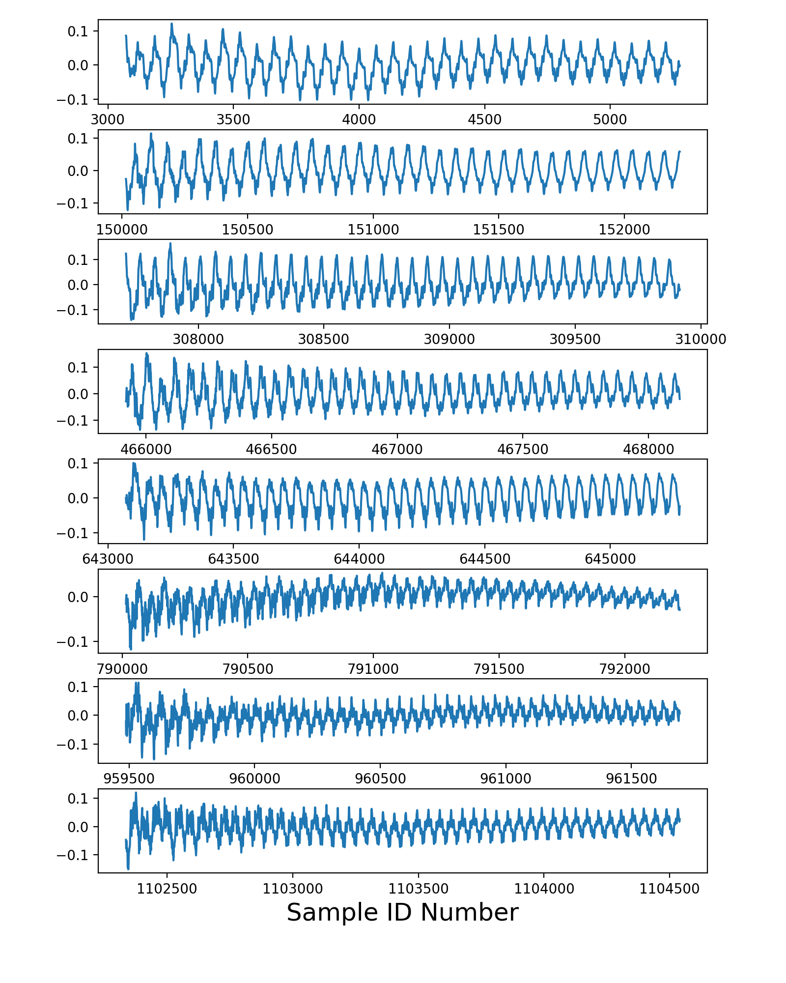
代码生成的第二个图形显示了自相关曲线，这是在freq_from_autocorr()函数内部计算的。垂直红线描绘了每个曲线左侧第一个峰值的位置，这是由peakutils软件包估计的。另一个开发人员使用的方法在某些红线上得到了不正确的结果；这就是为什么他的函数版本偶尔会返回错误的频率。

​

​

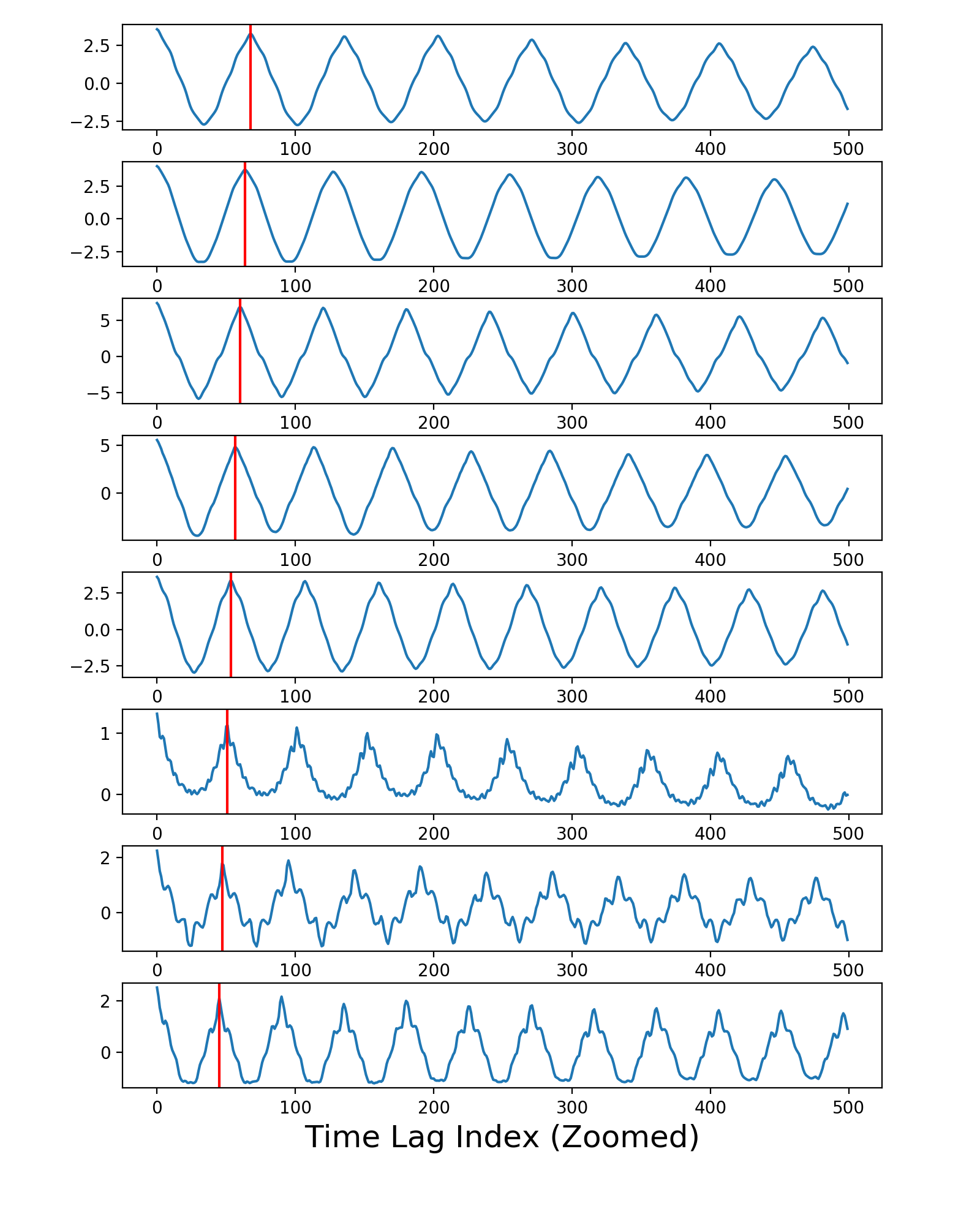
我的建议是在其他录音上测试freq_from_autocorr()函数的修订版，看看是否能找到更有挑战性的例子，即使是改进的版本也会给出不正确的结果，然后创造性地尝试开发一种更健壮的、永远不会出错的峰值查找算法。

Answer 2

自相关方法并不总是正确的。您可能希望实现一种更复杂的方法，如殷：

YIN.pdf

或MPM：

Pitch.pdf

以上两篇论文都读得很好。