在多个文件中使用ggplot绘制数据

Question

我有一个时间序列数据文件，有4种代谢产物A，B，AE和E的浓度随时间的变化。我有许多这种类型的数据文件(大约100个)。我想绘制一个图表中所有文件中所有四个代谢物的时间序列。每种代谢物都被指定为特定的颜色。

我编译了下面的代码，但是它只在一个文件(最后一个)中绘制数据。我认为这是因为当我调用ggplot()时，它会创建一个新的绘图。我试着在四个循环之外创建一个情节，但没有成功。

p = NULL

for(i in 1:length(filesToProcess)){
  fileName = filesToProcess[i]

  fileContent = read.csv(fileName)
  #fileContent$Time <- NULL

    p <- ggplot()+ 
    geom_line(data = fileContent, aes(x = Time, y = A, color = "A"), size =0.8) +
    geom_line(data = fileContent, aes(x = Time, y = B, color = "B"), size =0.8)  +
    geom_line(data = fileContent, aes(x = Time, y = AE, color = "AE"), size =0.8)  +
    geom_line(data = fileContent, aes(x = Time, y = E, color = "E"), size =0.8)  +
    xlab('Time') +
    ylab('Metabolite Concentration')+
    ggtitle('Step Scan') +
    labs(color="Metabolites")

}
plot(p)

下面是图

​

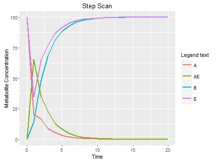
示例文件可以找到 here

Answer 1

我通常采用以下方法(未经测试，因为缺乏可重复的示例)

read_one <- function(f, ...){
  w <- read.csv(f, ...)
  m <- reshape2::melt(w, id = c("Time"))
  m$source <- tools::file_path_sans_ext(f) # keep track of filename
  m
}

plot_one <- function(d){
  ggplot(d, aes(x=Time, y=value)) + 
    geom_line(aes(colour=variable), size = 0.8) +
    ggtitle('Step Scan') +
    labs(x = 'Time', y = 'Metabolite Concentration', color="Metabolites")
}

## strategy 1 (multiple independent plots)

ml <- lapply(filesToProcess, read_one)
pl <- lapply(ml, plot_one)

gridExtra::grid.arrange(grobs = pl)

## strategy 2: facetting

m <- plyr::ldply(filesToProcess, read_one)
ggplot(m, aes(x=Time, y=value)) + 
  facet_wrap(~source) +
  geom_line(aes(colour=variable), size = 0.8) +
  ggtitle('Step Scan') +
  labs(x = 'Time', y = 'Metabolite Concentration', color="Metabolites")

Answer 2

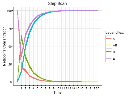
我想我解决了这个问题。我承认答案有点粗糙。但是，如果我能够在for循环之外初始化"p“变量，它就解决了这个问题。

filesToProcess = readLines("FilesToProcess.txt")

#initializing the variable with ggplot() object
p <- ggplot()

for(i in 1:length(filesToProcess)){
  fileName = filesToProcess[i]
  fileContent = read.csv(fileName)

  p <- p + 
  geom_line(data = fileContent, aes(x = Time, y = A, color = "A"), size =0.8) +
  geom_line(data = fileContent, aes(x = Time, y = B, color = "B"), size =0.8)  +
  geom_line(data = fileContent, aes(x = Time, y = AE, color = "AE"), size =0.8)  +
  geom_line(data = fileContent, aes(x = Time, y = E, color = "E"), size =0.8)

}

p <- p + theme_bw() + scale_x_continuous(breaks=1:20) + 
  xlab('Time') +
  ylab('Metabolite Concentration')+
  ggtitle('Step Scan') +
  labs(color="Legend text")
plot(p)

​

​