数据的指数拟合(python)

Question

嗨，我试图用多项式或指数函数来拟合我的数据，这两个函数都失败了。我使用的代码如下：

with open('argon.dat','r') as f:
    argon=f.readlines()

eng1 = np.array([float(argon[argon.index(i)].split('\n')[0].split('  ')[0])*1000 for i in argon])
II01 = np.array([1-math.exp(-float(argon[argon.index(i)].split('\n')[0].split('  ')[1])*(1.784e-3*6.35)) for i in argon])

with open('copper.dat','r') as f:
    copper=f.readlines()

eng2 = [float(copper[copper.index(i)].split('\n')[0].split('  ')[0])*1000 for i in copper]
II02 = [math.exp(-float(copper[copper.index(i)].split('\n')[0].split('  ')[1])*(8.128e-2*8.96)) for i in copper]

fig, ax1 = plt.subplots(figsize=(12,10))
ax2 = ax1.twinx()
ax1.set_yscale('log')
ax2.set_yscale('log')

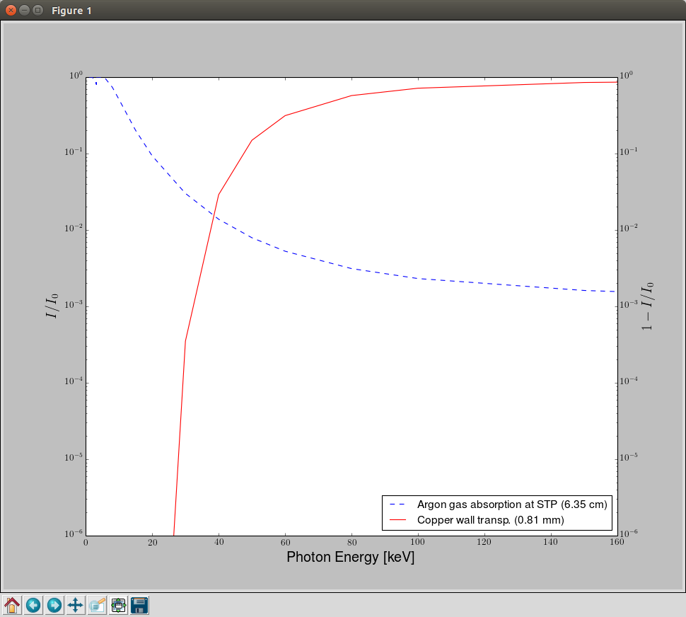
arg = ax2.plot(eng1, II01, 'b--', label='Argon gas absorption at STP (6.35 cm)')
cop = ax1.plot(eng2, II02, 'r', label='Copper wall transp. (0.81 mm)')
plot = arg+cop

labs = [l.get_label() for l in plot]
ax1.legend(plot,labs,loc='lower right', fontsize=14)
ax1.set_ylim(1e-6,1)
ax2.set_ylim(1e-6,1)
ax1.set_xlim(0,160)
ax1.set_ylabel(r'$\displaystyle I/I_0$', fontsize=18)
ax2.set_ylabel(r'$\displaystyle 1-I/I_0$', fontsize=18)
ax1.set_xlabel('Photon Energy [keV]', fontsize=18)
plt.show()

这给了我

我想要做的不是像这样绘制数据，把它们拟合成指数曲线，然后乘以这些曲线，得到检测器的效率(我试着逐个元素乘以，但我没有足够的数据点来获得光滑的曲线)，我尝试使用多重拟合，并且尝试定义一个指数函数来查看它是否工作，但是在这两种情况下，我最后都得到了一条线。

#def func(x, a, c, d):
#    return a*np.exp(-c*x)+d
#    
#popt, pcov = curve_fit(func, eng1, II01)
#plt.plot(eng1, func(eng1, *popt), label="Fitted Curve")

和

model = np.polyfit(eng1, II01 ,5) 
y = np.poly1d(model)
#splineYs = np.exp(np.polyval(model,eng1)) # also tried this but didnt work
ax2.plot(eng1,y)

在需要的情况下，从http://www.nist.gov/pml/data/xraycoef/index.cfm获取的数据也可以在图3：http://scitation.aip.org/content/aapt/journal/ajp/83/8/10.1119/1.4923022中找到类似的工作

“休息”是在“奥利弗”回答后进行的：

我使用已有的数据进行乘法：

i = 0
eff1 = []
while i < len(arg):
    eff1.append(arg[i]*cop[i])
    i += 1 

我最终得到的是(红色:铜，虚蓝色:氩，蓝色:乘法)

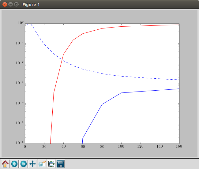
这就是我想要得到的，但通过使用曲线的函数，这将是一条光滑的曲线，我想得到它(在@oliver的回答中，关于哪里是错的或什么被误解了，我已经发表了评论)。

Answer 1

curvefit给您一个常量(一条平行线)的原因是，您正在传递一个使用您定义的模型不相关的数据集！

让我首先重新创建您的设置：

argon = np.genfromtxt('argon.dat')
copper = np.genfromtxt('copper.dat')

f1 = 1 - np.exp(-argon[:,1] * 1.784e-3 * 6.35)
f2 = np.exp(-copper[:,1] * 8.128e-2 * 8.96)

现在请注意，f1是基于argon.dat文件中数据的第二列。它与第一列无关，尽管没有什么可以阻止您绘制第二列与第一列的修改版本，当然，这就是您在绘图时所做的：

import matplotlib.pyplot as plt
from scipy.optimize import curve_fit

plt.semilogy(copper[:,0]*1000, f2, 'r-')  # <- f2 was not based on the first column of that file, but on the 2nd. Nothing stops you from plotting those together though...
plt.semilogy(argon[:,0]*1000, f1, 'b--')
plt.ylim(1e-6,1)
plt.xlim(0, 160)

def model(x, a, b, offset):
    return a*np.exp(-b*x) + offset

注意:在您的模型中，有一个名为b的参数是未使用的。这总是一个不好的想法传递给一个适当的算法。把它处理掉。

现在，诀窍是:使用指数模型，基于第二列制作了f1。因此，您应该传递curve_fit，第二列作为自变量(在函数的doc-string中标记为xdata )，然后传递f1作为因变量。如下所示：

popt1, pcov = curve_fit(model, argon[:,1], f1)
popt2, pcov = curve_fit(model, cupper[:,1], f2)

那会很好的。

现在，当您想要绘制这两个图的乘积的光滑版本时，您应该从自变量中的一个公共区间开始。对你来说，这就是光子能量。两个数据文件中的第二列都依赖于这一点:有一个函数(一个用于氩，另一个用于铜)，它将μ/ρ与光子能量联系起来。因此，如果您有大量用于能量的数据点，并且您成功地获得了这些函数，那么您将有许多用于μ/ρ的数据点。但是，由于这些函数是未知的，我能做的最好的事情就是简单地插值。但是，数据是对数的，所以需要对数插值，而不是默认的线性插值。

现在，继续获取光子能量的大量数据点。在数据集中，能量点呈指数增长，因此可以使用np.logspace创建一组像样的新点。

indep_var = argon[:,0]*1000
energy = np.logspace(np.log10(indep_var.min()),
                     np.log10(indep_var.max()),
                     512)  # both argon and cupper have the same min and max listed in the "energy" column.

这对我们的优势是，两个数据集中的能量具有相同的最小值和最大能量。否则，您将不得不缩小这个日志空间的范围。

接下来，我们(对数)插值关系energy -> μ/ρ。

interpolated_mu_rho_argon = np.power(10, np.interp(np.log10(energy), np.log10(indep_var), np.log10(argon[:,1]))) # perform logarithmic interpolation
interpolated_mu_rho_copper = np.power(10, np.interp(np.log10(energy), np.log10(copper[:,0]*1000), np.log10(copper[:,1])))

下面是刚才所做工作的可视化表示：

f, ax = plt.subplots(1,2, sharex=True, sharey=True)
ax[0].semilogy(energy, interpolated_mu_rho_argon, 'gs-', lw=1)
ax[0].semilogy(indep_var, argon[:,1], 'bo--', lw=1, ms=10)
ax[1].semilogy(energy, interpolated_mu_rho_copper, 'gs-', lw=1)
ax[1].semilogy(copper[:,0]*1000, copper[:,1], 'bo--', lw=1, ms=10)
ax[0].set_title('argon')
ax[1].set_title('copper')
ax[0].set_xlabel('energy (keV)')
ax[0].set_ylabel(r'$\mu/\rho$ (cm²/g)')

​

​

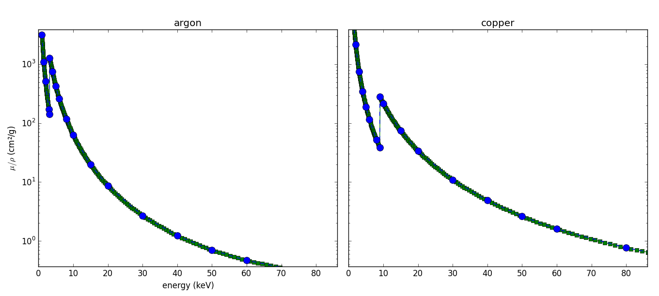
用蓝点标记的原始数据集已被精细内插。

现在，最后的步骤变得容易了。由于已经找到了将μ/ρ映射到某些指数型变量(我已重命名为f1和f2的函数)的模型参数，因此可以使用这些参数生成现有数据的平滑版本，以及这两个函数的乘积：

plt.figure()
plt.semilogy(energy, model(interpolated_mu_rho_argon, *popt1), 'b-', lw=1)
plt.semilogy(argon[:,0]*1000, f1, 'bo ')

plt.semilogy(copper[:,0]*1000, f2, 'ro ',)
plt.semilogy(energy, model(interpolated_mu_rho_copper, *popt2), 'r-', lw=1) # same remark here!

argon_copper_prod = model(interpolated_mu_rho_argon, *popt1)*model(interpolated_mu_rho_copper, *popt2)
plt.semilogy(energy, argon_copper_prod, 'g-')

plt.ylim(1e-6,1)
plt.xlim(0, 160)
plt.xlabel('energy (keV)')
plt.ylabel(r'$\mu/\rho$ (cm²/g)')

​

​

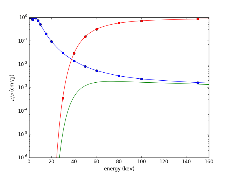
然后就到了。概括地说：

1. 生成足够数量的自变量数据点，以获得平滑的结果。
2. 插值关系photon energy -> μ/ρ
3. 将您的函数映射到插值的μ/ρ