比较速率-曲线和退化

Question

我有9个退化曲线，我想比较，并希望就如何最好地这样做的建议。我最初的想法是比较非线性回归。我会先解释这个问题，然后再详细说明实验设计：

我的问题是：

1. 我如何比较我的9个组之间的退化率？
2. 如何确定我的两个主要自变量(有机质类型和田间地块)在多大程度上推动了降解速度。

我在3个地块(A，B，C)中放置了3种类型的有机质(X，Y，Z)。每个样地放置12个有机质样品(每块36个样本，共108个样本)。我知道每个样品的原始有机物(包括总量和干物质百分比)的含量。在每周3个时间点(T1、T2、T3)，我从每块地块中取出每种类型的4个样品，并再次测量有机质含量。

因此，对于9种组合(AX，AY，AZ，BX，BY，CX，CY，CZ，CZ)中的每一种，我在T0有12种原始有机物测量，在后3个时间点(T1、T2、T3)各测量4种有机物。

我希望我提供了足够的信息我非常感谢围绕这个问题提供的任何帮助和建议。

谢谢，圣诞快乐。

安德鲁。

链接到示例日期：https://docs.google.com/spreadsheets/d/1a5w9BeeogprKAOwHi3WYSW7JF8EtjQOaaG9z-qzDRgw/pub?output=xlsx

Answer 1

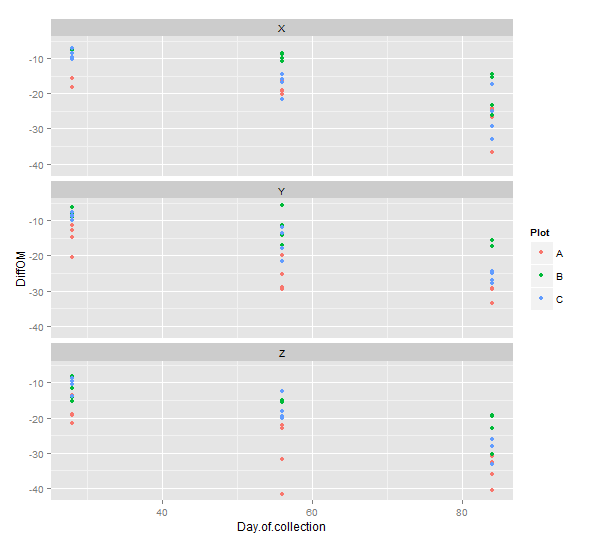
这里有件事可以很快给你一个开始。由于你的几个时间点，我会使用线性模型。在这里，我假设OM的绝对差异是合理的，即样品是以某种有意义的方式被规范化的。您可能需要使用相对值(在这种情况下甚至可能需要GLMM )。

library(data.table)
DT <- fread("Untitled spreadsheet.csv")
setnames(DT, make.names(names(DT)))
DT[, DiffOM := OM.at.collection..g. - Original.OM..T0...g.]
DT <- DT[-1]

library(ggplot2)
p <- ggplot(DT, aes(x = Day.of.collection, y = DiffOM, color = Plot)) +
  geom_point() +
  facet_wrap(~ Sample.type, ncol = 1)
print(p)

​

​

有些人建议，只有当有更多的群体可用时，才会有随机的拟合效果，但我通常相信，如果这样的拟合看起来合理的话，也会有少数几个组的模型。当然，在这种情况下，您不应该太相信随机效应的方差估计。或者，您可以将Plot看作是一个固定的效果，但是您的模型还需要另外两个参数。然而，通常我们对地块差异不太感兴趣，而更倾向于集中在处理效果上。YMMV

library(lmerTest)

fit1 <- lmer(DiffOM ~ Day.of.collection * Sample.type + (1 | Plot), data = DT)
fit2 <- lmer(DiffOM ~ Day.of.collection * Sample.type + (Day.of.collection | Plot), data = DT)
lme4:::anova.merMod(fit1, fit2)
#random slope doesn't really improve the model

fit3 <- lmer(DiffOM ~ Day.of.collection * Sample.type + (Sample.type | Plot), data = DT)
lme4:::anova.merMod(fit1, fit3)
#including the Sample type doesn't either

summary(fit1)
#apparently the interactions are far from significant

fit1a <- lmer(DiffOM ~ Day.of.collection + Sample.type + (1 | Plot), data = DT)
lme4:::anova.merMod(fit1, fit1a)
plot(fit1a)
#seems more or less okay with possibly exception of small degradation
#you could try a variance structure as implemented in package nlme

anova(fit1a)
#Analysis of Variance Table of type III  with  Satterthwaite 
#approximation for degrees of freedom
#                  Sum Sq Mean Sq NumDF DenDF F.value    Pr(>F)    
#Day.of.collection 3909.4  3909.4     1   102 222.145 < 2.2e-16 ***
#Sample.type        452.4   226.2     2   102  12.853 1.051e-05 ***
#---
#Signif. codes:  0 ‘***’ 0.001 ‘**’ 0.01 ‘*’ 0.05 ‘.’ 0.1 ‘ ’ 1

很明显，在样本类型之间，样本之前的退化率是不同的(参见根据样本类型而进行的不同截取)，这将意味着非线性速率(正如我们所预期的)。线性模型的差异意味着恒定的绝对退化率。

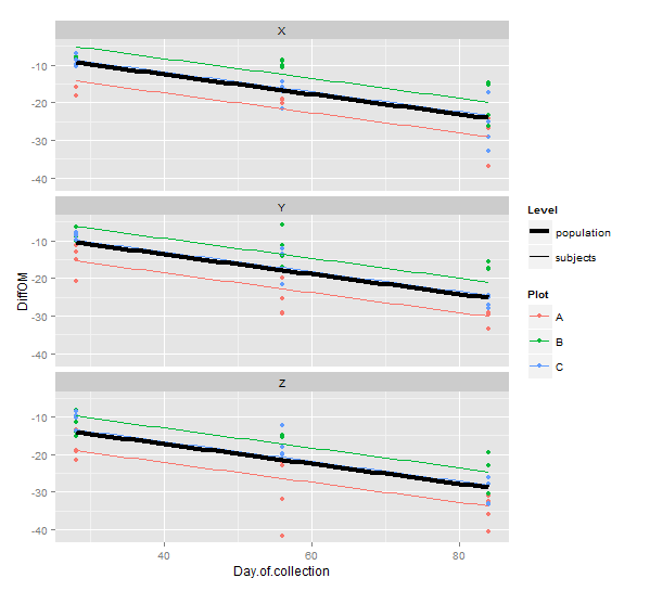
summary(fit1a)

newdat <- expand.grid(Day.of.collection = seq(28, 84, by = 1), 
                      Plot = c("A", "B", "C"), 
                      Sample.type = c("X", "Y", "Z"))
newdat$pred <- predict(fit1a, newdata = newdat)
newdat$pred0 <- predict(fit1a, newdata = newdat, re.form = NA)

p +
  geom_line(data = newdat, aes(y = pred, size = "subjects")) +
  geom_line(data = newdat, aes(y = pred0, size = "population", color = NULL)) +
  scale_size_manual(name = "Level",
                    values = c("subjects" = 0.5, "population" = 1.5))

​

​