选择光栅数据有效范围的最快方法

Question

使用R，我需要选择一个给定光栅的有效范围(从包raster)以最快的方式。我试过这个：

library(raster)
library(microbenchmark)
library(ggplot2)
library(compiler)

r <- raster(ncol=100, nrow=100)
r[] <- runif(ncell(r))

#Let's see if precompiling helps speed...
f <- function(x, min, max) reclassify(x, c(-Inf, min, NA, max, Inf, NA))
g <- cmpfun(f)

#Benchmark!
compare <- microbenchmark(
    calc(r, fun=function(x){ x[x < 0.2] <- NA; x[x > 0.8] <- NA; return(x)}), 
    reclassify(r, c(-Inf, 0.2, NA, 0.8, Inf, NA)),
    g(r, 0.2, 0.8),
    times=100)
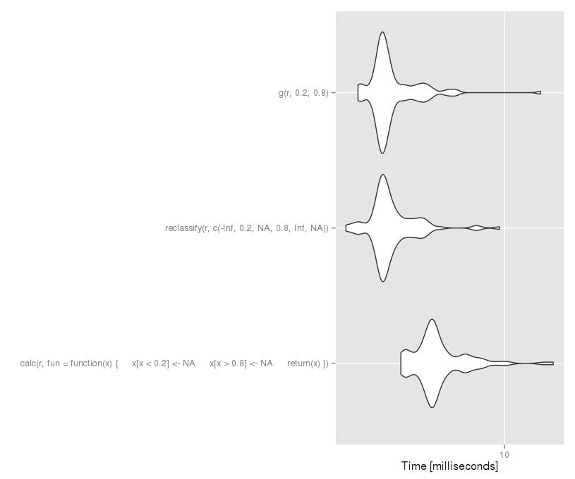
autoplot(compare) #Reclassify is much faster, precompiling doesn't help much.

#Check they are the same...
identical(
          calc(r, fun=function(x){ x[x < 0.2] <- NA; x[x > 0.8] <- NA; return(x)}),
          reclassify(r, c(-Inf, 0.2, NA, 0.8, Inf, NA))
) #TRUE
identical(
          reclassify(r, c(-Inf, 0.2, NA, 0.8, Inf, NA)),
          g(r, 0.2, 0.8),
) #TRUE

​

​

重分类方法要快得多，但我相信它可以加快速度。我怎样才能做到呢？

Answer 1

还有一种方法：

h <- function(r, min, max) {
  rr <- r[]
  rr[rr < min | rr > max] <- NA
  r[] <- rr
  r
}

i <- cmpfun(h)

identical(
  i(r, 0.2, 0.8),
  g(r, 0.2, 0.8)
)



#Benchmark!
compare <- microbenchmark(
  calc(r, fun=function(x){ x[x < 0.2] <- NA; x[x > 0.8] <- NA; return(x)}), 
  reclassify(r, c(-Inf, 0.2, NA, 0.8, Inf, NA)),
  g(r, 0.2, 0.8),
  h(r, 0.2, 0.8),
  i(r, 0.2, 0.8),
  times=100)
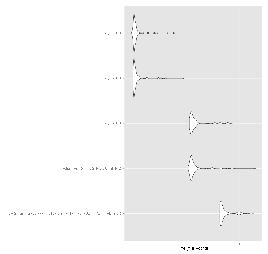
autoplot(compare) 

编译在这种情况下没有多大帮助。

​

​

您甚至可以通过直接使用@访问光栅对象的插槽来进一步提高速度(尽管通常不鼓励这样做)。

j <- function(r, min, max) {
  v <- r@data@values
  v[v < min | v > max] <- NA
  r@data@values <- v
  r
}

k <- cmpfun(j)

identical(
  j(r, 0.2, 0.8)[],
  g(r, 0.2, 0.8)[]
)

​

​

Answer 2

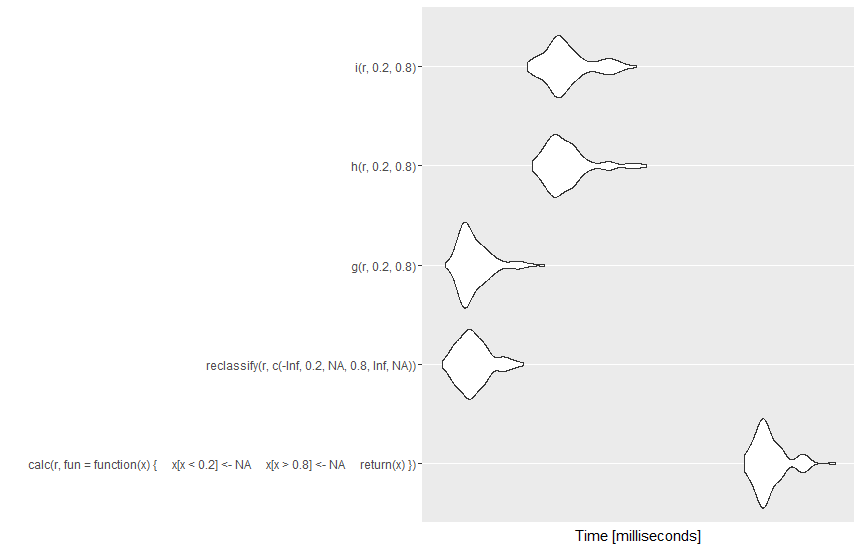
虽然对这个问题的公认答案对于光栅来说是正确的，但重要的是要注意，最快的安全函数高度依赖光栅大小：@rengis提供的函数h和i只有相对较小的栅格(和相对简单的重分类)才更快。在OP的示例中，只需将光栅r的大小增加10级，就可以使reclassify更快：

# Code from OP @AF7
library(raster)
library(microbenchmark)
library(ggplot2)
library(compiler)

#Let's see if precompiling helps speed...
f <- function(x, min, max) reclassify(x, c(-Inf, min, NA, max, Inf, NA))
g <- cmpfun(f)

# Funcions from @rengis
h <- function(r, min, max) {
  rr <- r[]
  rr[rr < min | rr > max] <- NA
  r[] <- rr
  r
}

i <- cmpfun(h)

# Benchmark with larger raster (100k cells, vs 10k originally)
r <- raster(ncol = 1000, nrow = 100)
r[] <- runif(ncell(r))

compare <- microbenchmark(
  calc(r, fun=function(x){ x[x < 0.2] <- NA; x[x > 0.8] <- NA; return(x)}), 
  reclassify(r, c(-Inf, 0.2, NA, 0.8, Inf, NA)),
  g(r, 0.2, 0.8),
  h(r, 0.2, 0.8),
  i(r, 0.2, 0.8),
  times=100)
autoplot(compare) 

​

​

reclassify变得更快的确切点既取决于栅格中细胞的数量，也取决于重新分类的复杂性，但在这种情况下，交叉点大约在50,000个单元格(见下文)。

随着光栅变得更大(或者计算更复杂)，另一种加快重新分类的方法是使用多线程，例如使用snow包：

# Reclassify, using clusterR to split into two threads
library(snow)
tryCatch({
      beginCluster(n = 2)
      clusterR(r, reclassify, args = list(rcl = c(-Inf, 0.2, NA, 0.8, Inf, NA)))
    }, finally = endCluster())

多线程涉及到更多的设置开销，因此只有在非常大的栅格和/或更复杂的计算中才有意义(事实上，我惊讶地注意到，在我下面测试过的任何条件下，它都不是最好的选择--也许是进行更复杂的重新分类？)

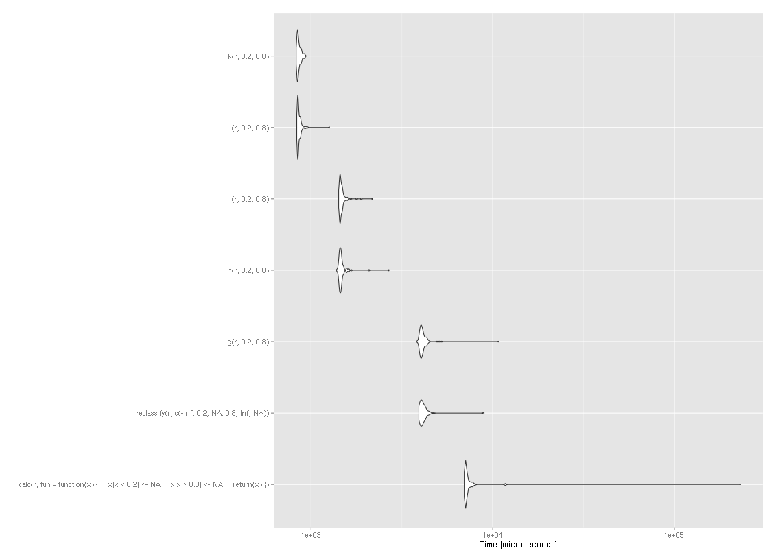
为了举例说明，我用OP的设置间隔了1,000万个单元(每个单元运行10次)，绘制了微基准测试的结果如下：

​

​

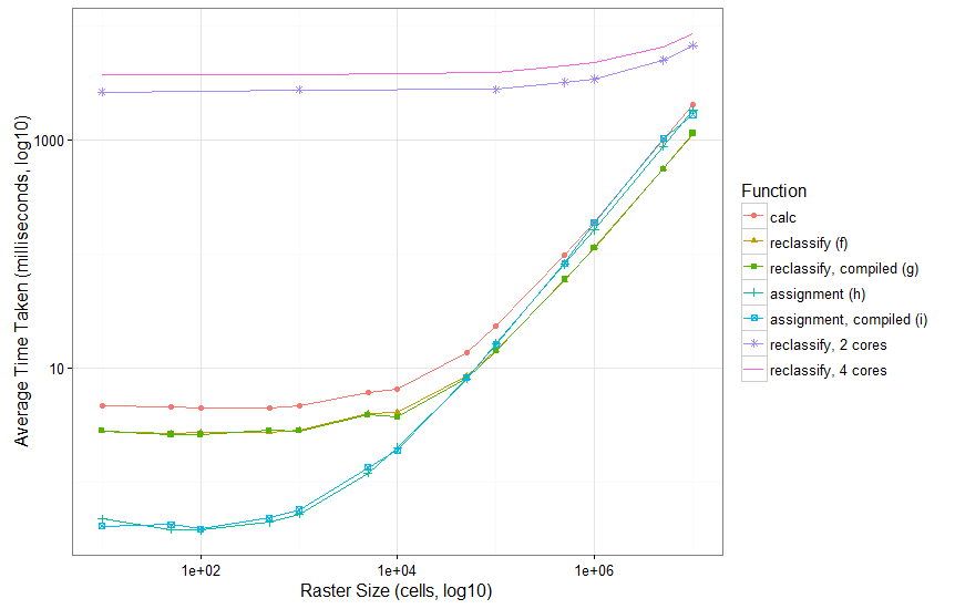
作为最后的说明，编译在任何测试大小上都没有区别。

Answer 3

光栅包具有这样的功能：clamp。它比g快，但比h和i慢，因为它内置了一些开销(安全性)。

compare <- microbenchmark(
  h(r, 0.2, 0.8),
  i(r, 0.2, 0.8),
  clamp(r, 0.2, 0.8),
  g(r, 0.2, 0.8),
  times=100)
autoplot(compare)