零膨胀泊松模型不适合

Question

以下是数据和设置：

library(fitdistrplus)
library(gamlss)

finalVector <- dput(finalVector)
c(0, 0, 0, 0, 0, 0, 0, 0, 0, 0, 0, 0, 0, 0, 0, 0, 0, 0, 0, 0, 
0, 0, 0, 0, 0, 0, 0, 0, 0, 0, 0, 0, 0, 0, 0, 0, 0, 0, 0, 0, 0, 
0, 0, 0, 0, 0, 0, 0, 0, 0, 0, 0, 0, 0, 0, 0, 0, 0, 0, 0, 0, 0, 
0, 0, 0, 0, 0, 0, 0, 0, 0, 0, 0, 0, 0, 0, 0, 0, 0, 0, 0, 0, 0, 
0, 0, 2, 1, 1, 1, 1, 1, 1, 1, 1, 2, 2, 2, 1, 2, 1, 1, 1, 1, 1, 
1, 1, 2, 1, 1, 2, 1, 1, 1, 1, 2, 1, 3, 2, 1, 1, 1, 1, 1, 1, 2, 
2, 1, 4, 2, 3, 1, 2, 3, 1, 1, 1, 1, 1, 1, 1, 1, 1, 1, 1, 1, 1, 
2, 1, 2, 2, 1, 1, 4, 1, 2, 2, 1, 1, 1, 1, 1, 2, 1, 1, 2, 2, 1, 
2, 1, 1, 4, 2, 2, 1, 1, 2, 1, 1, 1, 1, 1, 1)

countFitPoisson <- fitdist(finalVector,"pois",  method = "mle", lower = 0)
countFitZeroPoisson <- fitdist(finalVector, 'ZIP', start = list( ##mu  = mean of poisson, sigma = prob(x = 0))
                                                           mu = as.numeric(countFitPoisson$estimate), 
                                                            sigma = as.numeric(as.numeric(countFitPoisson$estimate))
                                                          ), method = "mle", lower= 0) 

第一次调用成功。决赛说没能估计，我不知道原因。谢谢!

编辑：

假设我正确地完成了代码(不确定)，那么我唯一能想到的就是没有足够的零来适应模型？

Answer 1

你的数据并不是零膨胀的，因此拟合模型不会导致改进.我使用的不是fitdistr方法，而是下面的glm和扩展回归模型。所有回归(子)模型只是使用一个常量(或拦截)，但没有任何真正的回归者。为了实现可视化，我通过package提供的countreg包(其中包含pscl计数数据回归的后续函数)使用rootograms。

首先，让我们看看Poisson fit：

(mp <- glm(finalVector ~ 1, family = poisson))
## Call:  glm(formula = finalVector ~ 1, family = poisson)
## 
## Coefficients:
## (Intercept)  
##      -0.284  
## 
## Degrees of Freedom: 181 Total (i.e. Null);  181 Residual
## Null Deviance:      200.2 
## Residual Deviance: 200.2        AIC: 418.3

这相当于exp(-0.284)的拟合平均值，即约0.753。如果您比较观察到的频率和拟合的频率，这非常符合数据：

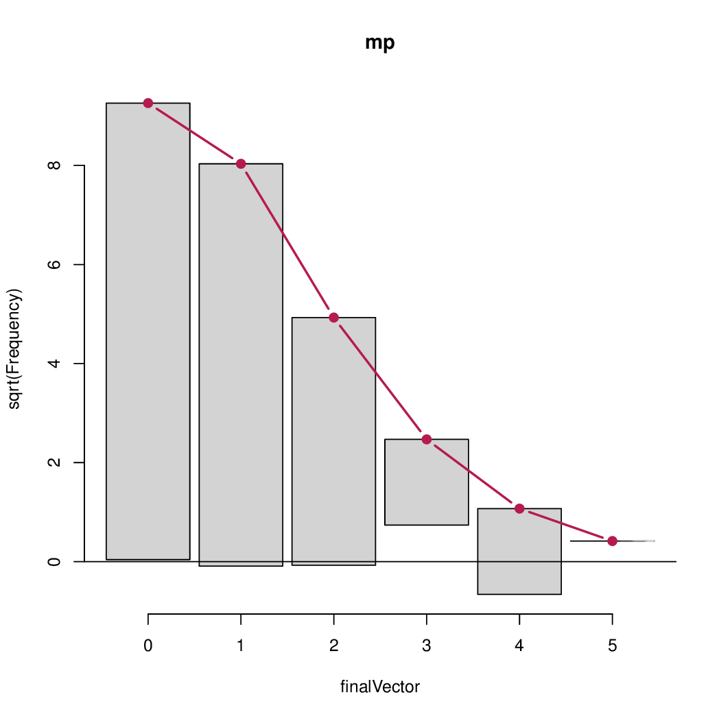
library("countreg")
rootogram(mp)

这表明，对于计数0，1，2的拟合基本上是完美的，只有3，4，5的小偏差，但这些频率无论如何都是非常低的。因此，从这一点来看，似乎没有必要对模型进行扩展。

​

​

但要与其他模型进行正式比较，人们可以考虑零膨胀泊松(正如你尝试过的)一个障碍泊松或负二项式。零膨胀模型的结果是：

(mzip <- zeroinfl(finalVector ~ 1 | 1, dist = "poisson"))
## Call:
## zeroinfl(formula = finalVector ~ 1 | 1, dist = "poisson")
## 
## Count model coefficients (poisson with log link):
## (Intercept)  
##     -0.2839  
## 
## Zero-inflation model coefficients (binomial with logit link):
## (Intercept)  
##      -9.151  

因此，计数平均数与以前基本相同，零通货膨胀的概率基本为零(plogis(-9.151)约为0.01%)。

该跨栏模型工作类似，但可以使用零删失泊松模型的0-vs-更大和截断泊松的正计数。然后，这也嵌套在Poisson模型中，因此Wald测试可以很容易地进行：

mhp <- hurdle(finalVector ~ 1 | 1, dist = "poisson", zero.dist = "poisson")
hurdletest(mhp)
## Wald test for hurdle models
## 
## Restrictions:
## count_((Intercept) - zero_(Intercept) = 0
## 
## Model 1: restricted model
## Model 2: finalVector ~ 1 | 1
## 
##   Res.Df Df Chisq Pr(>Chisq)
## 1    181                    
## 2    180  1 0.036     0.8495

这也清楚地表明，没有多余的零和一个简单的泊松模型就足够了。

作为最后的检查，还可以考虑一个负二项分布模型：

(mnb <- glm.nb(finalVector ~ 1))
## Call:  glm.nb(formula = finalVector ~ 1, init.theta = 125.8922776, link = log)
## 
## Coefficients:
## (Intercept)  
##      -0.284  
## 
## Degrees of Freedom: 181 Total (i.e. Null);  181 Residual
## Null Deviance:      199.1 
## Residual Deviance: 199.1        AIC: 420.3

这又是一个几乎相同的平均值和一个巨大的θ参数，足够接近无穷大(= Poisson)。因此，总的来说，Poisson模型是足够的，不需要任何考虑的扩展。可能性几乎没有变化，附加参数(零通胀、零门槛、θ-色散)也没有任何改善：

AIC(mp, mzip, mhp, mnb)
##      df      AIC
## mp    1 418.2993
## mzip  2 420.2996
## mhp   2 420.2631
## mnb   2 420.2959