
谱图是否显示正确的值?
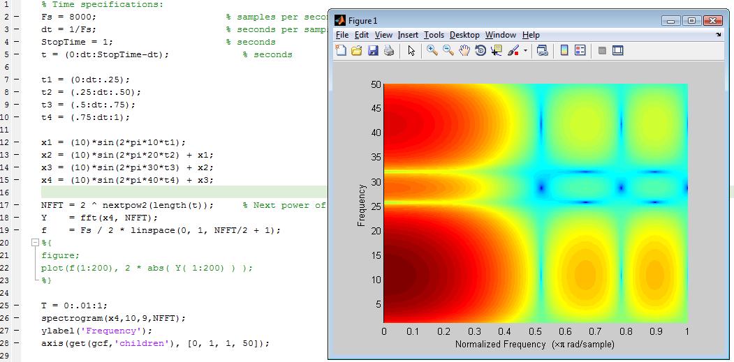
我想知道下面发布的spectrogram是否是给定的非平稳信号的真实表示。
如果这是一个真实的表现,我有一些问题,关于情节的具体特征.
对于水平轴上的0->.25,为什么它会显示最高频率的信号分量?我假设,给定第一次持续时间t1,我应该只看到信号x1的频率。此外,鉴于第二次持续时间t2,我应该只看到信号x2的频率,等等。但是,这不是我在下面发布的spectrogram中看到的。
你能解释一下为什么我们在光谱图上看到这些特征吗?
带方程的谱图
码
% Time specifications:
Fs = 8000;                       % samples per second
dt = 1/Fs;                       % seconds per sample
StopTime = 1;                    % seconds
t = (0:dt:StopTime-dt);             % seconds

t1 = (0:dt:.25);
t2 = (.25:dt:.50);
t3 = (.5:dt:.75);
t4 = (.75:dt:1);

 x1 = (10)*sin(2*pi*10*t1);
x2 = (10)*sin(2*pi*20*t2) + x1;
x3 = (10)*sin(2*pi*30*t3) + x2;
x4 = (10)*sin(2*pi*40*t4) + x3;


NFFT = 2 ^ nextpow2(length(t));     % Next power of 2 from length of y
Y    = fft(x4, NFFT);
f    = Fs / 2 * linspace(0, 1, NFFT/2 + 1);
%{
figure;
plot(f(1:200), 2 * abs( Y( 1:200) ) );
%}

 T = 0:.01:1;
 spectrogram(x4,10,9,NFFT);
 ylabel('Frequency');
axis(get(gcf,'children'), [0, 1, 1, 50]);Update_1:当我尝试建议的答案时,我收到了以下信息。
??? Out of memory. Type HELP MEMORY for your options.
Error in ==> spectrogram at 168
y = y(1:length(f),:);
Error in ==> stft_1 at 36
spectrogram(x,10,9,NFFT);
所用的守则:
% Time specifications:
Fs = 8000;                       % samples per second
dt = 1/Fs;                       % seconds per sample
StopTime = 1;                    % seconds
t = (0:dt:StopTime-dt);             % seconds

%get a full-length example of each signal component
x1 = (10)*sin(2*pi*10*t);
x2 = (10)*sin(2*pi*20*t);
x3 = (10)*sin(2*pi*30*t);
x4 = (10)*sin(2*pi*40*t);

%construct a composite signal
x = zeros(size(t));
I = find((t >= t1(1)) & (t <= t1(end)));
x(I) = x1(I);
I = find((t >= t2(1)) & (t <= t2(end)));
x(I) = x2(I);
I = find((t >= t3(1)) & (t <= t3(end)));
x(I) = x3(I);
I = find((t >= t4(1)) & (t <= t4(end)));
x(I) = x4(I);

NFFT = 2 ^ nextpow2(length(t));     % Next power of 2 from length of y
Y    = fft(x, NFFT);
f    = Fs / 2 * linspace(0, 1, NFFT/2 + 1);
%{
figure;
plot(f(1:200), 2 * abs( Y( 1:200) ) );
 %}

T = 0:.01:1;
spectrogram(x,10,9,NFFT);
ylabel('Frequency');
  axis(get(gcf,'children'), [0, 1, 1, 50]);
Update_2
% Time specifications:
Fs = 8000;                       % samples per second
dt = 1/Fs;                       % seconds per sample
 StopTime = 1;                    % seconds
  t = (0:dt:StopTime-dt);             % seconds
  t1 = ( 0:dt:.25);
  t2 = (.25:dt:.50);
  t3 = (.5:dt:.75);
  t4 = (.75:dt:1);

  %get a  full-length example of each signal component
 x1 = (10)*sin(2*pi*100*t);
 x2 = (10)*sin(2*pi*200*t);
 x3 = (10)*sin(2*pi*300*t);
 x4 = (10)*sin(2*pi*400*t);

 %construct a composite signal
 x = zeros(size(t));
 I = find((t >= t1(1)) & (t <= t1(end)));
 x(I) = x1(I);
 I = find((t >= t2(1)) & (t <= t2(end)));
 x(I) = x2(I);
 I = find((t >= t3(1)) & (t <= t3(end)));
 x(I) = x3(I);
 I = find((t >= t4(1)) & (t <= t4(end)));
 x(I) = x4(I);

 NFFT = 2 ^ nextpow2(length(t));     % Next power of 2 from length of y
 Y    = fft(x, NFFT);
 f    = Fs / 2 * linspace(0, 1, NFFT/2 + 1);
 %{
 figure;
 plot(f(1:200), 2 * abs( Y( 1:200) ) );
 %}

 T = 0:.001:1;
 spectrogram(x,10,9);
 ylabel('Frequency');
axis(get(gcf,'children'), [0, 1, 1, 100]);Dpectrogram_2:
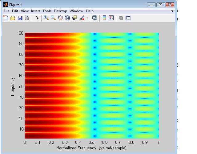
回答 1
Stack Overflow用户
发布于 2014-12-31 02:08:49
我不认为你在策划你认为你在策划的事情。您应该在时域中绘制信号,以确保它看起来像您所期望的.plot(x4)。我认为你认为你的信号是x1,x2,x3,x4。然而,根据您正在展示的Matlab代码,情况并非如此。
相反,您的信号是x1+x2+x3+x4在彼此之上的总和。因此,您应该看到信号分量在10,20,30,40赫兹,以及其他组成部分,因为瞬态启动的信号。
为了得到你想要的信号,你应该做如下的事情:
%get a full-length example of each signal component
t = (0:dt:StopTime-dt);
x1 = (10)*sin(2*pi*10*t);
x2 = (10)*sin(2*pi*20*t);
x3 = (10)*sin(2*pi*30*t);
x4 = (10)*sin(2*pi*40*t);

%construct a composite signal from the four signals above
x = zeros(size(t)); %allocate an empty vector of the correct size
I = find((t >= t1(1)) & (t <= t1(end)));
x(I) = x1(I);
I = find((t >= t2(1)) & (t <= t2(end)));
x(I) = x2(I);
I = find((t >= t3(1)) & (t <= t3(end)));
x(I) = x3(I);
I = find((t >= t4(1)) & (t <= t4(end)));
x(I) = x4(I);
然后,您可以在时域( x )绘制新的信号plot(x),以确保这是您想要的。最后,您可以执行您的spectrogram。
请注意,在每个时间段之间( t1和t2之间,t2和t3之间,然后在t3和t4之间)过渡时,您将在光谱图中看到工件。信号伪影将反映在不同信号频率之间的不连续过渡期间信号是复杂的。
https://stackoverflow.com/questions/27708690
复制相似问题
腾讯云开发者

Copyright © 2013 - 2026 Tencent Cloud. All Rights Reserved. 腾讯云 版权所有
深圳市腾讯计算机系统有限公司 ICP备案/许可证号:粤B2-20090059 ![]() 粤公网安备44030502008569号
粤公网安备44030502008569号
腾讯云计算(北京)有限责任公司 京ICP证150476号 | 京ICP备11018762号