高斯混合模型(GMM)

Question

我一直在玩Scikit-learn的GMM功能。首先，我沿着x=y创建了一个发行版。

from sklearn import mixture
import numpy as np 
import matplotlib.pyplot as plt
from mpl_toolkits.mplot3d import Axes3D

line_model = mixture.GMM(n_components = 99)
#Create evenly distributed points between 0 and 1.
xs = np.linspace(0, 1, 100)
ys = np.linspace(0, 1, 100)

#Create a distribution that's centred along y=x
line_model.fit(zip(xs,ys))
plt.plot(xs, ys)
plt.show()

这就产生了预期的分布：

​

接下来，我给出了一个GMM，并绘制了结果：

#Create the x,y mesh that will be used to make a 3D plot
x_y_grid = []
for x in xs:
    for y in ys:
        x_y_grid.append([x,y])

#Calculate a probability for each point in the x,y grid.
x_y_z_grid = []
for x,y in x_y_grid:
    z = line_model.score([[x,y]])
    x_y_z_grid.append([x,y,z])

x_y_z_grid = np.array(x_y_z_grid)

#Plot probabilities on the Z axis.
fig = plt.figure()
ax = fig.gca(projection='3d')
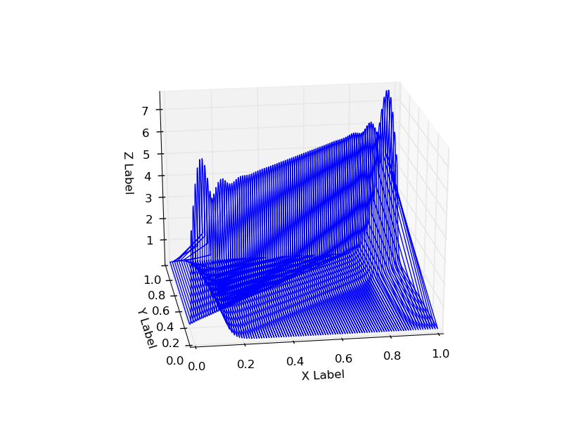
ax.plot(x_y_z_grid[:,0], x_y_z_grid[:,1], 2.72**x_y_z_grid[:,2])
plt.show()

结果的概率分布沿x=0和x=1有一些奇怪的尾，在拐角上也有额外的概率(x=1、y=1和x=0、y=0)。

​

使用n_components=5还显示了这种行为：

​

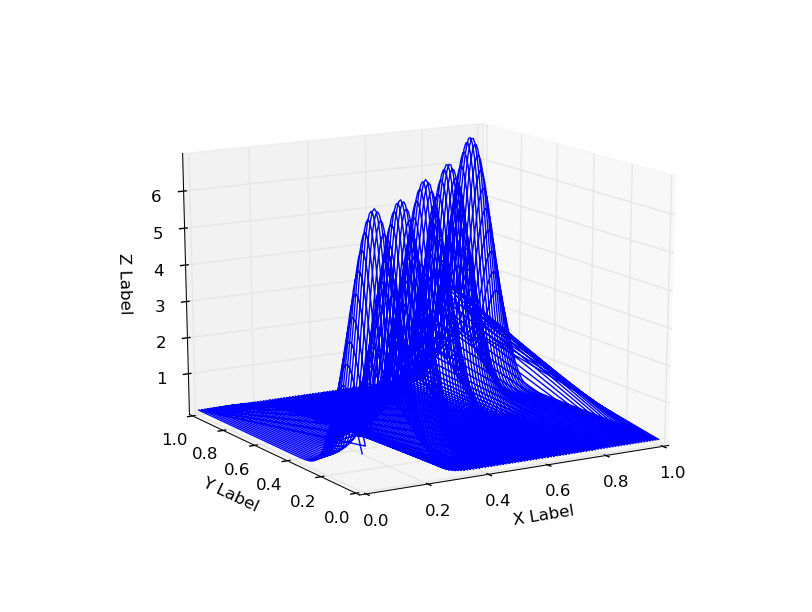
这是GMM固有的问题，还是实现存在问题，还是我做错了什么？

编辑:从模型中获得分数似乎可以摆脱这种行为--这应该是吗？

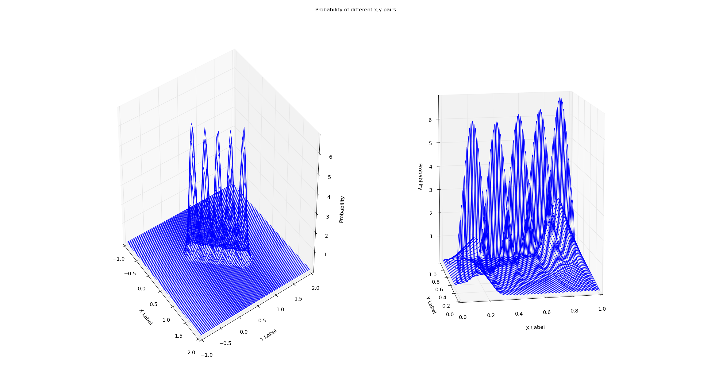
我正在同一数据集上训练这两个模型(从x=y到x=0到x=1)。通过gmm的score方法对概率进行简单的检验，可以消除这种边界效应。为什么会这样呢？我已经附上了下面的情节和代码。

​

​

# Creates a line of 'observations' between (x_small_start, x_small_end)
# and (y_small_start, y_small_end). This is the data both gmms are trained on.
x_small_start = 0
x_small_end = 1
y_small_start = 0
y_small_end = 1

# These are the range of values that will be plotted
x_big_start = -1
x_big_end = 2
y_big_start = -1
y_big_end = 2


shorter_eval_range_gmm = mixture.GMM(n_components = 5)
longer_eval_range_gmm = mixture.GMM(n_components = 5)

x_small = np.linspace(x_small_start, x_small_end, 100)
y_small = np.linspace(y_small_start, y_small_end, 100)
x_big = np.linspace(x_big_start, x_big_end, 100)
y_big = np.linspace(y_big_start, y_big_end, 100)

#Train both gmms on a distribution that's centered along y=x
shorter_eval_range_gmm.fit(zip(x_small,y_small))
longer_eval_range_gmm.fit(zip(x_small,y_small))


#Create the x,y meshes that will be used to make a 3D plot
x_y_evals_grid_big = []
for x in x_big:
    for y in y_big:
        x_y_evals_grid_big.append([x,y])
x_y_evals_grid_small = []

for x in x_small:
    for y in y_small:
        x_y_evals_grid_small.append([x,y])

#Calculate a probability for each point in the x,y grid.
x_y_z_plot_grid_big = []
for x,y in x_y_evals_grid_big:
    z = longer_eval_range_gmm.score([[x, y]])
    x_y_z_plot_grid_big.append([x, y, z])
x_y_z_plot_grid_big = np.array(x_y_z_plot_grid_big)

x_y_z_plot_grid_small = []
for x,y in x_y_evals_grid_small:
    z = shorter_eval_range_gmm.score([[x, y]])
    x_y_z_plot_grid_small.append([x, y, z])
x_y_z_plot_grid_small = np.array(x_y_z_plot_grid_small)


#Plot probabilities on the Z axis.
fig = plt.figure()
fig.suptitle("Probability of different x,y pairs")

ax1 = fig.add_subplot(1, 2, 1, projection='3d')
ax1.plot(x_y_z_plot_grid_big[:,0], x_y_z_plot_grid_big[:,1], np.exp(x_y_z_plot_grid_big[:,2]))
ax1.set_xlabel('X Label')
ax1.set_ylabel('Y Label')
ax1.set_zlabel('Probability')
ax2 = fig.add_subplot(1, 2, 2, projection='3d')
ax2.plot(x_y_z_plot_grid_small[:,0], x_y_z_plot_grid_small[:,1], np.exp(x_y_z_plot_grid_small[:,2]))
ax2.set_xlabel('X Label')
ax2.set_ylabel('Y Label')
ax2.set_zlabel('Probability')

plt.show()

Answer 1

没有问题的契合，但你正在使用的可视化。提示应该是连接(0,1,5)到(0,1,0)的直线，这实际上只是两个点的连接的呈现(这是由于读取点的顺序所致)。虽然这两个极端点都在你的数据中，但实际上这条线上没有其他点。

就我个人而言，我认为使用3d图(线)来表示表面是一个非常糟糕的主意，因为上面提到的原因，我建议用表面图或等高线图代替。

试试这个：

from sklearn import mixture
import numpy as np 
import matplotlib.pyplot as plt
from mpl_toolkits.mplot3d import Axes3D

line_model = mixture.GMM(n_components = 99)
#Create evenly distributed points between 0 and 1.
xs = np.atleast_2d(np.linspace(0, 1, 100)).T
ys = np.atleast_2d(np.linspace(0, 1, 100)).T

#Create a distribution that's centred along y=x
line_model.fit(np.concatenate([xs, ys], axis=1))
plt.scatter(xs, ys)
plt.show()

#Create the x,y mesh that will be used to make a 3D plot
X, Y = np.meshgrid(xs, ys)
x_y_grid = np.c_[X.ravel(), Y.ravel()]

#Calculate a probability for each point in the x,y grid.
z = line_model.score(x_y_grid)
z = z.reshape(X.shape)

#Plot probabilities on the Z axis.
fig = plt.figure()
ax = fig.add_subplot(111, projection='3d')
ax.plot_surface(X, Y, z)
plt.show()

从学术角度来看，我对用二维混合模型在二维空间中拟合一维线的目标感到很不舒服。GMM的流形学习至少需要法线方向具有零方差，从而减少到dirac分布。从数值和分析上看，这是不稳定的，应该避免(在gmm拟合中似乎存在一些稳定技巧，因为模型的方差在法向直线方向上相当大)。

在绘制数据时，还建议使用plt.scatter而不是plt.plot，因为在拟合这些点的联合分布时，没有理由将它们连接起来。

希望这有助于了解你的问题。