快速、优雅的经验/样本协方差函数计算方法

Question

如果可能的话，有没有人知道用Python计算经验/样本协方差函数的好方法？

这是一个书的屏幕截图，其中包含了covariagram的一个很好的定义：

​

​

如果我正确地理解了它，对于给定的滞后/宽度h，我应该得到由h(或小于h)分隔的所有对点，乘以它的值，并对每一个点计算它的平均值，在这种情况下，它被定义为m(x_i)。然而，根据m(x_{i})的定义，如果要计算m( x1 )，则需要得到距离x1在h以内的值的平均值。这看起来是一个非常密集的计算。

首先，我是否正确理解了这一点？如果是这样的话，假设是二维空间，什么是计算这个的好方法呢？我试着用Python (使用numpy和熊猫)来编写这个代码，但是它需要几秒钟时间，我甚至不确定它是否正确，这就是为什么我不在这里发布代码的原因。下面是另一次非常幼稚的实现尝试：

from scipy.spatial.distance import pdist, squareform
distances = squareform(pdist(np.array(coordinates))) # coordinates is a nx2 array
z = np.array(z) # z are the values
cutoff = np.max(distances)/3.0 # somewhat arbitrary cutoff
width = cutoff/15.0
widths = np.arange(0, cutoff + width, width)
Z = []
Cov = []

for w in np.arange(len(widths)-1): # for each width
    # for each pairwise distance
    for i in np.arange(distances.shape[0]): 
        for j in np.arange(distances.shape[1]): 
            if distances[i, j] <= widths[w+1] and distances[i, j] > widths[w]:
                m1 = []
                m2 = []
                # when a distance is within a given width, calculate the means of
                # the points involved
                for x in np.arange(distances.shape[1]):
                    if distances[i,x] <= widths[w+1] and distances[i, x] > widths[w]:
                        m1.append(z[x])

                for y in np.arange(distances.shape[1]):
                    if distances[j,y] <= widths[w+1] and distances[j, y] > widths[w]:
                        m2.append(z[y])

                mean_m1 = np.array(m1).mean() 
                mean_m2 = np.array(m2).mean()
                Z.append(z[i]*z[j] - mean_m1*mean_m2)
    Z_mean = np.array(Z).mean() # calculate covariogram for width w
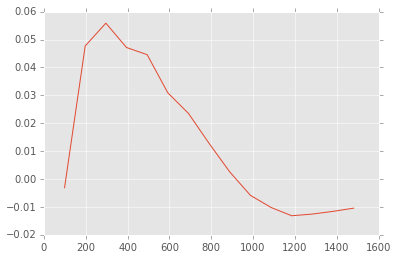
    Cov.append(Z_mean) # collect covariances for all widths

但是，现在我已经确认代码中有一个错误。我知道，因为我用变异函数来计算协变函数(协方差图(H)=协方差函数(0)-变异函数(H))，我得到了一个不同的图：

​

​

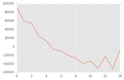
它应该是这样的：

​

​

最后，如果你知道一个Python/R/MATLAB库来计算经验协变函数，请告诉我。至少这样我就能证实我做了什么。

Answer 1

我们可以使用scipy.cov，但是如果直接进行计算(这非常容易)，有更多的方法来加快速度。

首先，制作一些具有一定空间相关性的假数据。我首先要做的是做空间相关性，然后使用使用它生成的随机数据点，其中数据是根据底层地图定位的，并且还接受底层地图的值。

编辑1:

我改变了数据点生成器，使位置是纯粹随机的，但z值与空间地图成正比。而且，我改变了地图，使左右两面相对于彼此移动，从而在大范围的h中产生负相关性。

from numpy import *
import random
import matplotlib.pyplot as plt

S = 1000
N = 900
# first, make some fake data, with correlations on two spatial scales
#     density map
x = linspace(0, 2*pi, S)
sx = sin(3*x)*sin(10*x)
density = .8* abs(outer(sx, sx))
density[:,:S//2] += .2
#     make a point cloud motivated by this density
random.seed(10)  # so this can be repeated
points = []
while len(points)<N:
    v, ix, iy = random.random(), random.randint(0,S-1), random.randint(0,S-1)
    if True: #v<density[ix,iy]:
        points.append([ix, iy, density[ix,iy]])
locations = array(points).transpose()
print locations.shape
plt.imshow(density, alpha=.3, origin='lower')
plt.plot(locations[1,:], locations[0,:], '.k')
plt.xlim((0,S))
plt.ylim((0,S))
plt.show()
#     build these into the main data: all pairs into distances and z0 z1 values
L = locations
m = array([[math.sqrt((L[0,i]-L[0,j])**2+(L[1,i]-L[1,j])**2), L[2,i], L[2,j]] 
                         for i in range(N) for j in range(N) if i>j])

这意味着：

​

​

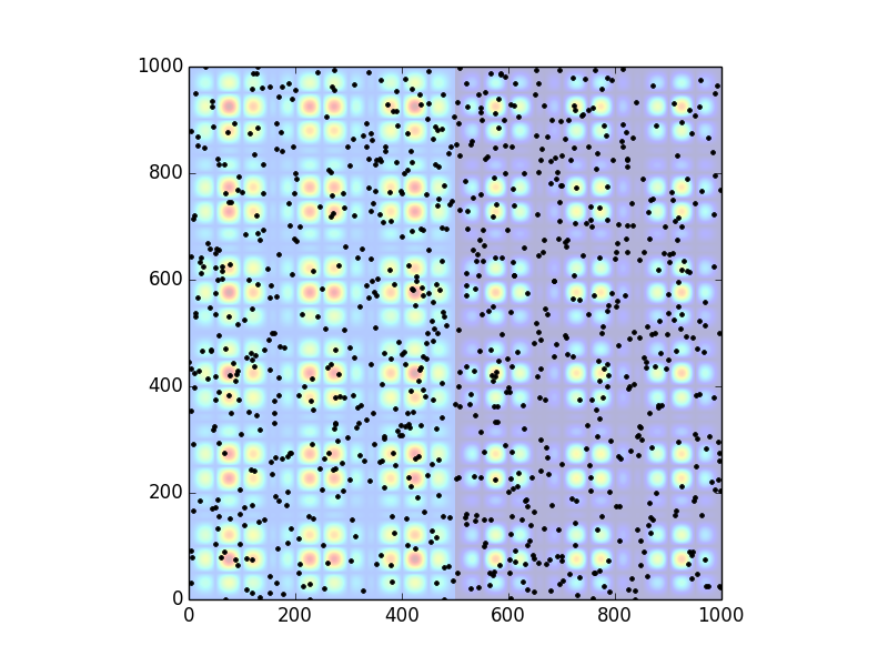
以上只是模拟的数据，我没有尝试优化它的生产，等等。我假设这是OP开始的地方，下面的任务，因为数据已经存在于实际情况中。

现在计算“协变函数”(这比生成假数据容易得多，顺便说一下)。这里的想法是通过h对所有对和相关值进行排序，然后使用ihvals对它们进行索引。也就是说，对索引ihval的求和是方程中N(h)上的和，因为这包括了hs低于所需值的所有对。

编辑2:

正如下面的注释中所建议的，N(h)现在只是h-dh和h之间的对，而不是0和h之间的所有对( dh是ihvals中h-values的间距--即下面使用的S/1000 )。

# now do the real calculations for the covariogram
#    sort by h and give clear names
i = argsort(m[:,0])  # h sorting
h = m[i,0]
zh = m[i,1]
zsh = m[i,2]
zz = zh*zsh

hvals = linspace(0,S,1000)  # the values of h to use (S should be in the units of distance, here I just used ints)
ihvals = searchsorted(h, hvals)
result = []
for i, ihval in enumerate(ihvals[1:]):
    start, stop = ihvals[i-1], ihval
    N = stop-start
    if N>0:
        mnh = sum(zh[start:stop])/N
        mph = sum(zsh[start:stop])/N
        szz = sum(zz[start:stop])/N
        C = szz-mnh*mph
        result.append([h[ihval], C])
result = array(result)
plt.plot(result[:,0], result[:,1])
plt.grid()
plt.show()

​

​

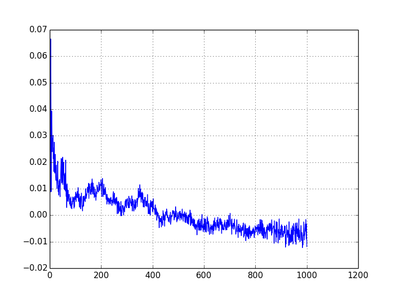
这在我看来是合理的，因为人们可以在h值的预期值处看到颠簸或低谷，但我没有仔细检查。

scipy.cov的主要加速是可以预先计算所有的产品，zz。否则，就会将zh和zsh输入到cov中，每一个新的h，并且所有的产品都将被重新计算。这个计算可以通过在每一个时间步长( ihvals[n-1] )到ihvals[n] (从n )进行部分求和来加速，但我怀疑这是必要的。