在分面ggplot2图中独立地定位两个传说

Question

我有一个由ggplot2生成的情节，其中包含两个传说。传说的位置并不理想，所以我想调整它们。我一直试图模仿the answer to "How do I position two legends independently in ggplot"中显示的方法。答案中所示的例子起作用了。然而，我无法得到所描述的方法来适应我的情况。

我使用R2.15.3 (2013-03-01)，ggplot2_0.9.3.1，点阵0.20-13，gtable_0.1.2，gridExtra_0.9.1对Debian挤压.

考虑一下minimal.R生成的图。这和我的实际情节很相似。

########################
minimal.R
########################

get_stat <- function()
  {
    n = 20
    q1 = qnorm(seq(3, 17)/20, 14, 5)
    q2 = qnorm(seq(1, 19)/20, 65, 10)
    Stat = data.frame(value = c(q1, q2),
      pvalue = c(dnorm(q1, 14, 5)/max(dnorm(q1, 14, 5)), d = dnorm(q2, 65, 10)/max(dnorm(q2, 65, 10))),
      variable = c(rep('true', length(q1)), rep('data', length(q2))))
    return(Stat)
  }

stat_all<- function()
{
  library(ggplot2)
  library(gridExtra)
  stathuman = get_stat()
  stathuman$dataset = "human"
  statmouse = get_stat()
  statmouse$dataset = "mouse"
  stat = merge(stathuman, statmouse, all=TRUE)
  return(stat)
}

simplot <- function()
  {
    Stat = stat_all()
    Pvalue = subset(Stat, variable=="true")
    pdf(file = "CDF.pdf", width = 5.5, height = 2.7)
    stat = ggplot() + stat_ecdf(data=Stat, n=1000, aes(x=value, colour = variable)) +
      theme(legend.key = element_blank(), legend.background = element_blank(), legend.position=c(.9, .25), legend.title = element_text(face = "bold")) +
        scale_x_continuous("Negative log likelihood") +
          scale_y_continuous("Proportion $<$ x") +
            facet_grid(~ dataset, scales='free') +
              scale_colour_manual(values = c("blue", "red"), name="Data type",
                                  labels=c("Gene segments", "Model"), guide=guide_legend(override.aes = list(size = 2))) +
                geom_area(data=Pvalue, aes(x=value, y=pvalue, fill=variable), position="identity", alpha=0.5) +
                  scale_fill_manual(values = c("gray"), name="Pvalue", labels=c(""))
    print(stat)
    dev.off()
  }

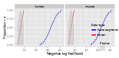
simplot()

这将导致下面的情节。可以看出，Data type和Pvalue传说的位置并不好。我将此代码修改为minimal2.R。

​

​

使用版本1，它应该将图例放在顶部，代码运行时没有错误，但没有显示图例。

编辑:有两个框显示，一个在另一个之上。上面那个是空白的。如果我不像@巴普蒂斯特所建议的那样在grid.arrange()中设定高度，那么传说和情节都会放在底部的盒子里。如果我设置的高度如图所示，那我就看不到传说了。

EDIT2:看起来额外的空白框是由grid.newpage调用的，我是从前面的问题中复制的。我不知道它为什么会在那里。如果我不使用那一行，那么我只得到一个框/页。

在版本2中，我得到了这个错误。

Error in UseMethod("grid.draw") :
  no applicable method for 'grid.draw' applied to an object of class "c('gg', 'ggplot')"
Calls: simplot -> grid.draw

编辑:如果我按照@baptiste的建议使用print(plotNew)，那么我将得到以下错误

Error in if (empty(data)) { : missing value where TRUE/FALSE needed 
Calls: simplot ... facet_map_layout -> facet_map_layout.grid -> locate_grid.

我试图弄清楚这是怎么回事，但我找不到多少相关的信息。

备注：

1. 我不知道为什么我要得到经验民防的楼梯效应。我肯定有一个很明显的解释。如果你知道的话请告诉我。
2. 如果有人能提出替代方案，例如matplotlib，我从未认真尝试过，我愿意考虑使用这种代码的替代品，甚至ggplot2来生成这个图。
3. 添加 打印(ggplot_gtable(ggplot_build(Stat2) minimal2.R给我的 TableGrob (7x7)“布局”：12个grobs z单元格名为grob 1 0 (1-7,1-7)背景矩形.背景.背景.矩形.186 2 1 (3-3,4-4)条-顶层绝对grobs.绝对值135 3 (3-3,6-6)条.顶绝对grobs.AbteGrob.141 4 5 (4-4,3-3)轴-l绝对GrobGRID.AbteGrob.129 53 (4-4,4-4)面板gTreeGRID.gTree.155 6 4 (4-4,6-6)面板gTreeGRID.gTree.169 7 6 (5-5,4-4)轴-b绝对Grob.117 8 (5-5,6-6)轴-b-绝对GrobID.AbteGrob.123 9 8(6-6-6) xlab出租车。Title.x.text.171 10 9(4-4,2-2) Ylabtextaxis.Title.y.text.173 11 10 (4-4,4-6)指南-方框gtableguide-方框12 11 (2-2,4-6)标题textplot.title.text.184 我不明白这是什么故障。有人能解释吗？guide-box是否与传说相对应，人们如何知道这一点？

下面是我的代码minimal2.R的修改版本。

########################
minimal2.R
########################

get_stat <- function()
  {
    n = 20
    q1 = qnorm(seq(3, 17)/20, 14, 5)
    q2 = qnorm(seq(1, 19)/20, 65, 10)
    Stat = data.frame(value = c(q1, q2),
      pvalue = c(dnorm(q1, 14, 5)/max(dnorm(q1, 14, 5)), d = dnorm(q2, 65, 10)/max(dnorm(q2, 65, 10))),
      variable = c(rep('true', length(q1)), rep('data', length(q2))))
    return(Stat)
  }

stat_all<- function()
{
  library(ggplot2)
  library(gridExtra)
  library(gtable)
  stathuman = get_stat()
  stathuman$dataset = "human"
  statmouse = get_stat()
  statmouse$dataset = "mouse"
  stat = merge(stathuman, statmouse, all=TRUE)
  return(stat)
}

simplot <- function()
  {
    Stat = stat_all()
    Pvalue = subset(Stat, variable=="true")
    pdf(file = "CDF.pdf", width = 5.5, height = 2.7)

    ## only include data type legend
    stat1 = ggplot() + stat_ecdf(data=Stat, n=1000, aes(x=value, colour = variable)) +
      theme(legend.key = element_blank(), legend.background = element_blank(), legend.position=c(.9, .25), legend.title = element_text(face = "bold")) +
        scale_x_continuous("Negative log likelihood") +
          scale_y_continuous("Proportion $<$ x") +
            facet_grid(~ dataset, scales='free') +
              scale_colour_manual(values = c("blue", "red"), name="Data type", labels=c("Gene segments", "Model"), guide=guide_legend(override.aes = list(size = 2))) +
                geom_area(data=Pvalue, aes(x=value, y=pvalue, fill=variable), position="identity", alpha=0.5) +
                  scale_fill_manual(values = c("gray"), name="Pvalue", labels=c(""), guide=FALSE)

    ## Extract data type legend
    dataleg <- gtable_filter(ggplot_gtable(ggplot_build(stat1)), "guide-box")

    ## only include pvalue legend
    stat2 = ggplot() + stat_ecdf(data=Stat, n=1000, aes(x=value, colour = variable)) +
      theme(legend.key = element_blank(), legend.background = element_blank(), legend.position=c(.9, .25), legend.title = element_text(face = "bold")) +
        scale_x_continuous("Negative log likelihood") +
          scale_y_continuous("Proportion $<$ x") +
            facet_grid(~ dataset, scales='free') +
              scale_colour_manual(values = c("blue", "red"), name="Data type", labels=c("Gene segments", "Model"), guide=FALSE) +
                geom_area(data=Pvalue, aes(x=value, y=pvalue, fill=variable), position="identity", alpha=0.5) +
                  scale_fill_manual(values = c("gray"), name="Pvalue", labels=c(""))

    ## Extract pvalue legend
    pvalleg <- gtable_filter(ggplot_gtable(ggplot_build(stat2)), "guide-box")

    ## no legends
    stat = ggplot() + stat_ecdf(data=Stat, n=1000, aes(x=value, colour = variable)) +
      theme(legend.key = element_blank(), legend.background = element_blank(), legend.position=c(.9, .25), legend.title = element_text(face = "bold")) +
        scale_x_continuous("Negative log likelihood") +
          scale_y_continuous("Proportion $<$ x") +
            facet_grid(~ dataset, scales='free') +
              scale_colour_manual(values = c("blue", "red"), name="Data type", labels=c("Gene segments", "Model"), guide=FALSE) +
                geom_area(data=Pvalue, aes(x=value, y=pvalue, fill=variable), position="identity", alpha=0.5) +
                  scale_fill_manual(values = c("gray"), name="Pvalue", labels=c(""), guide=FALSE)

    ## Add data type legend: version 1 (data type legend should be on top)
    ## plotNew <- arrangeGrob(dataleg, stat, heights = unit.c(dataleg$height, unit(1, "npc") - dataleg$height), ncol = 1)

    ## Add data type legend: version 2 (data type legend should be somewhere in the interior)
    ## plotNew <- stat + annotation_custom(grob = dataleg, xmin = 7, xmax = 10, ymin = 0, ymax = 4)

    grid.newpage()
    grid.draw(plotNew)
    dev.off()
  }

simplot()

Answer 1

这可以用grid.arrange和arrangeGrob来完成，但是正确地调整高度和宽度是很痛苦的。

grid.arrange(arrangeGrob(dataleg, pvalleg, nrow=1, ncol=2, widths=c(unit(1, "npc"), unit(5, "cm"))), stat, nrow=2, heights=c(unit(.2, "npc"), unit(.8, "npc")))

我通常更喜欢用一个合适的图例来制作一个新的情节，并使用这个新的传说：

 h <- ggplot(data.frame(a=rnorm(10), b=rnorm(10), c=factor(rbinom(10, 1,.5), labels=c("Gene segments", "Model")), d=factor("")), 
        aes(x=a, y=b)) +
   geom_line(aes(color=c), size=1.3) + geom_polygon(aes(fill=d)) +
   scale_color_manual(values=c("blue", "red"), name="Data type") + 
   scale_fill_manual(values="gray", name="P-value") 
 g_legend<-function(a.gplot){
   tmp <- ggplot_gtable(ggplot_build(a.gplot))
   leg <- which(sapply(tmp$grobs, function(x) x$name) == "guide-box")
   legend <- tmp$grobs[[leg]]
   return(legend)
 }
 legend <- g_legend(h)

 grid.arrange(stat, legend, nrow=1, ncol=2, widths=c(unit(.8, "npc"), unit(.2, "npc")))
 grid.arrange(legend, stat, nrow=2, ncol=1, heights=c(unit(.2, "npc"), unit(.8, "npc")))