R中的流图？

Question

如何在R中实现流图？

流图是叠加图的一个变体，它在基线选择、层序和颜色选择方面对哈弗雷等人的ThemeRiver进行了改进。

示例：

​

​

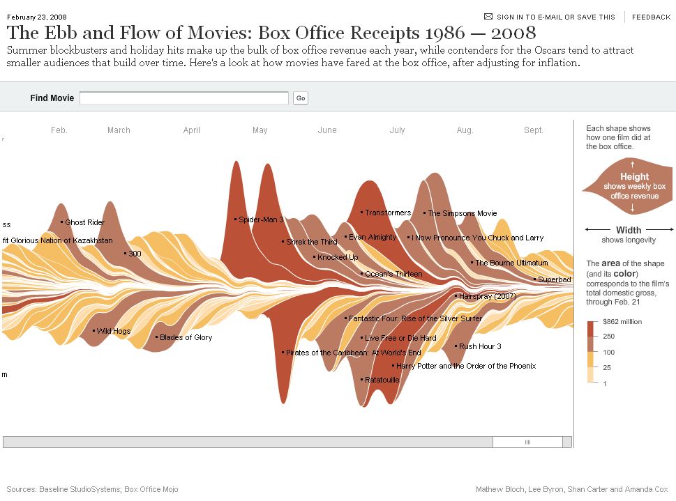
参考资料：http://www.leebyron.com/else/streamgraph/

Answer 1

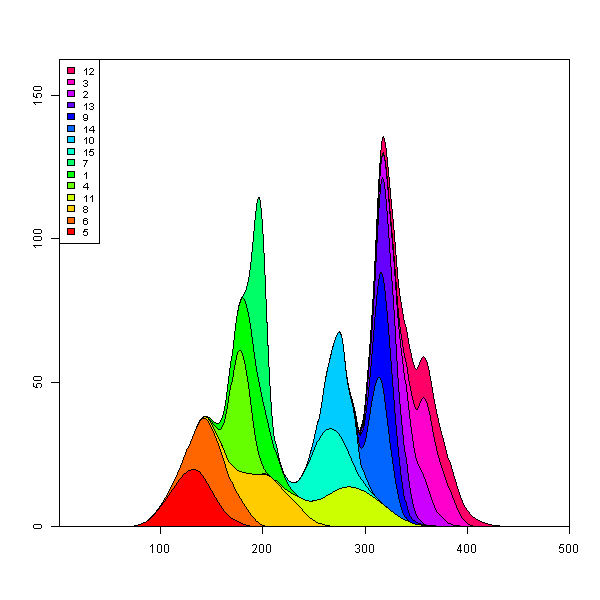
不久前，我编写了一个函数plot.stacked，它可以帮助您解决问题。

其职能是：

plot.stacked <- function(x,y, ylab="", xlab="", ncol=1, xlim=range(x, na.rm=T), ylim=c(0, 1.2*max(rowSums(y), na.rm=T)), border = NULL, col=rainbow(length(y[1,]))){

    plot(x,y[,1], ylab=ylab, xlab=xlab, ylim=ylim, xaxs="i", yaxs="i", xlim=xlim, t="n")
    bottom=0*y[,1]
    for(i in 1:length(y[1,])){
        top=rowSums(as.matrix(y[,1:i]))
        polygon(c(x, rev(x)), c(top, rev(bottom)), border=border, col=col[i])
        bottom=top
    }
    abline(h=seq(0,200000, 10000), lty=3, col="grey")
    legend("topleft", rev(colnames(y)), ncol=ncol, inset = 0, fill=rev(col), bty="0", bg="white", cex=0.8, col=col)
    box()
}

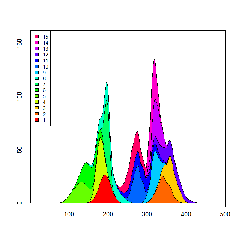
下面是一个示例数据集和一个绘图：

set.seed(1)
m <- 500
n <- 15
x <- seq(m)
y <- matrix(0, nrow=m, ncol=n)
colnames(y) <- seq(n)
for(i in seq(ncol(y))){
    mu <- runif(1, min=0.25*m, max=0.75*m)
    SD <- runif(1, min=5, max=30)
    TMP <- rnorm(1000, mean=mu, sd=SD)
    HIST <- hist(TMP, breaks=c(0,x), plot=FALSE)
    fit <- smooth.spline(HIST$counts ~ HIST$mids)
    y[,i] <- fit$y
}

    plot.stacked(x,y)

​

​

我可以想象，你只需要调整多边形“底部”的定义，就能得到你想要的情节。

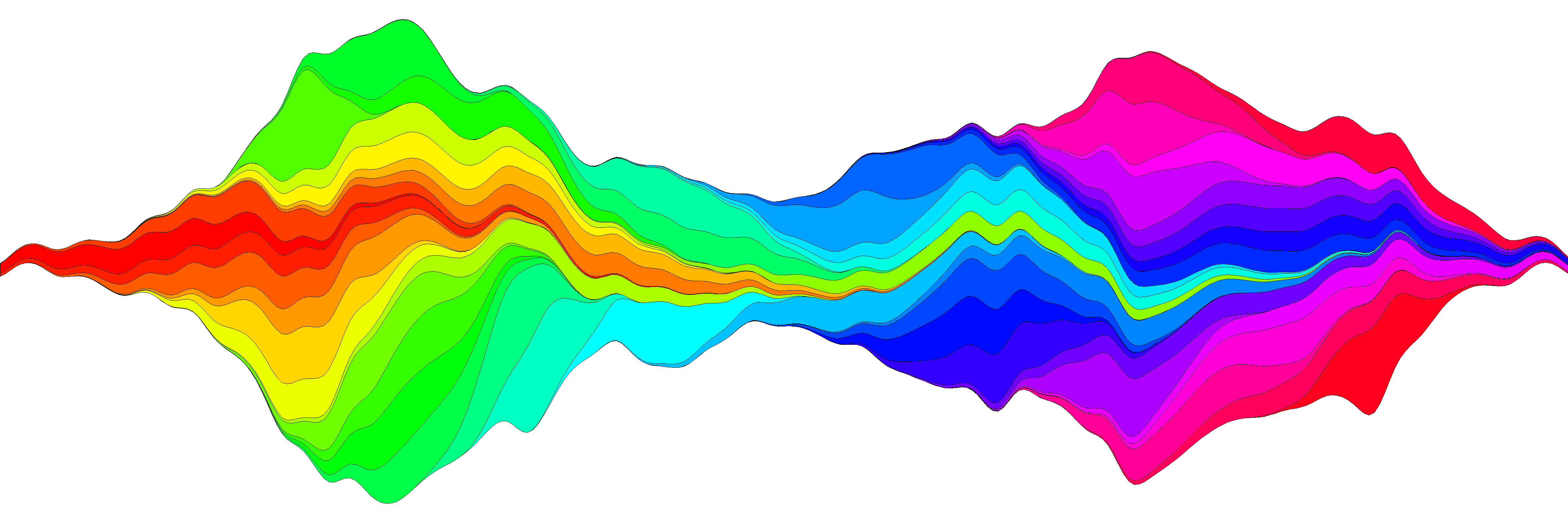
更新：

我在制作流图方面又做了一次尝试，并且相信我或多或少地在函数plot.stream中复制了这个想法，可用的在这个要点里，也复制到了这篇文章的底部。在此链接上，我将详细介绍它的使用情况，但下面是一个基本示例：

library(devtools)
source_url('https://gist.github.com/menugget/7864454/raw/f698da873766347d837865eecfa726cdf52a6c40/plot.stream.4.R')

set.seed(1)
m <- 500
n <- 50
x <- seq(m)
y <- matrix(0, nrow=m, ncol=n)
colnames(y) <- seq(n)
for(i in seq(ncol(y))){
    mu <- runif(1, min=0.25*m, max=0.75*m)
    SD <- runif(1, min=5, max=30)
    TMP <- rnorm(1000, mean=mu, sd=SD)
    HIST <- hist(TMP, breaks=c(0,x), plot=FALSE)
    fit <- smooth.spline(HIST$counts ~ HIST$mids)
    y[,i] <- fit$y
}
y <- replace(y, y<0.01, 0)

#order by when 1st value occurs
ord <- order(apply(y, 2, function(r) min(which(r>0))))
y2 <- y[, ord]
COLS <- rainbow(ncol(y2))

png("stream.png", res=400, units="in", width=12, height=4)
par(mar=c(0,0,0,0), bty="n")
plot.stream(x,y2, axes=FALSE, xlim=c(100, 400), xaxs="i", center=TRUE, spar=0.2, frac.rand=0.1, col=COLS, border=1, lwd=0.1)
dev.off()

​

​

plot.stream()代码

#plot.stream makes a "stream plot" where each y series is plotted 
#as stacked filled polygons on alternating sides of a baseline.
#
#Arguments include:
#'x' - a vector of values
#'y' - a matrix of data series (columns) corresponding to x
#'order.method' = c("as.is", "max", "first") 
#  "as.is" - plot in order of y column
#  "max" - plot in order of when each y series reaches maximum value
#  "first" - plot in order of when each y series first value > 0
#'center' - if TRUE, the stacked polygons will be centered so that the middle,
#i.e. baseline ("g0"), of the stream is approximately equal to zero. 
#Centering is done before the addition of random wiggle to the baseline. 
#'frac.rand' - fraction of the overall data "stream" range used to define the range of
#random wiggle (uniform distrubution) to be added to the baseline 'g0'
#'spar' - setting for smooth.spline function to make a smoothed version of baseline "g0"
#'col' - fill colors for polygons corresponding to y columns (will recycle)
#'border' - border colors for polygons corresponding to y columns (will recycle) (see ?polygon for details)
#'lwd' - border line width for polygons corresponding to y columns (will recycle)
#'...' - other plot arguments
plot.stream <- function(
    x, y, 
    order.method = "as.is", frac.rand=0.1, spar=0.2,
    center=TRUE,
    ylab="", xlab="",  
    border = NULL, lwd=1, 
    col=rainbow(length(y[1,])),
    ylim=NULL, 
    ...
){

if(sum(y < 0) > 0) error("y cannot contain negative numbers")

if(is.null(border)) border <- par("fg")
border <- as.vector(matrix(border, nrow=ncol(y), ncol=1))
col <- as.vector(matrix(col, nrow=ncol(y), ncol=1))
lwd <- as.vector(matrix(lwd, nrow=ncol(y), ncol=1))

if(order.method == "max") {
    ord <- order(apply(y, 2, which.max))
    y <- y[, ord]
    col <- col[ord]
    border <- border[ord]
}

if(order.method == "first") {
    ord <- order(apply(y, 2, function(x) min(which(r>0))))
    y <- y[, ord]
    col <- col[ord]
    border <- border[ord]
}

bottom.old <- rep(0, length(x))
top.old <- rep(0, length(x))
polys <- vector(mode="list", ncol(y))
for(i in seq(polys)){
    if(i %% 2 == 1){ #if odd
        top.new <- top.old + y[,i]
        polys[[i]] <- list(x=c(x, rev(x)), y=c(top.old, rev(top.new)))
        top.old <- top.new
    }
    if(i %% 2 == 0){ #if even
        bottom.new <- bottom.old - y[,i]
        polys[[i]] <- list(x=c(x, rev(x)), y=c(bottom.old, rev(bottom.new)))
        bottom.old <- bottom.new
    }
}

ylim.tmp <- range(sapply(polys, function(x) range(x$y, na.rm=TRUE)), na.rm=TRUE)
outer.lims <- sapply(polys, function(r) rev(r$y[(length(r$y)/2+1):length(r$y)]))
mid <- apply(outer.lims, 1, function(r) mean(c(max(r, na.rm=TRUE), min(r, na.rm=TRUE)), na.rm=TRUE))

#center and wiggle
if(center) {
    g0 <- -mid + runif(length(x), min=frac.rand*ylim.tmp[1], max=frac.rand*ylim.tmp[2])
} else {
    g0 <- runif(length(x), min=frac.rand*ylim.tmp[1], max=frac.rand*ylim.tmp[2])
}

fit <- smooth.spline(g0 ~ x, spar=spar)

for(i in seq(polys)){
    polys[[i]]$y <- polys[[i]]$y + c(fitted(fit), rev(fitted(fit)))
}

if(is.null(ylim)) ylim <- range(sapply(polys, function(x) range(x$y, na.rm=TRUE)), na.rm=TRUE)
plot(x,y[,1], ylab=ylab, xlab=xlab, ylim=ylim, t="n", ...)
for(i in seq(polys)){
    polygon(polys[[i]], border=border[i], col=col[i], lwd=lwd[i])
}

}

Answer 2

这些天来，有一个流htmlwidget：

https://hrbrmstr.github.io/streamgraph/

devtools::install_github("hrbrmstr/streamgraph")

library(streamgraph)

streamgraph(data, key, value, date, width = NULL, height = NULL,
  offset = "silhouette", interpolate = "cardinal", interactive = TRUE,
  scale = "date", top = 20, right = 40, bottom = 30, left = 50)

它产生了非常漂亮的图表，甚至是交互式的。

​

编辑

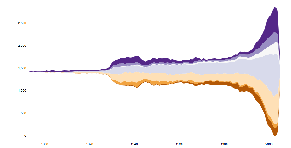
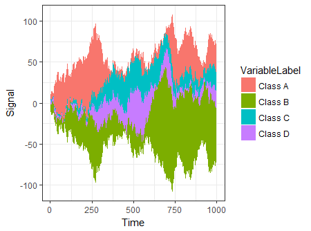
另一个选项是使用ggTimeSeries，它使用ggplot2的语法：

# creating some data
library(ggTimeSeries)
library(ggplot2)

set.seed(10)
dfData = data.frame(
   Time = 1:1000,
   Signal = abs(
      c(
         cumsum(rnorm(1000, 0, 3)), 
         cumsum(rnorm(1000, 0, 4)), 
         cumsum(rnorm(1000, 0, 1)),
         cumsum(rnorm(1000, 0, 2))
      )
   ),
   VariableLabel = c(rep('Class A', 1000),
                     rep('Class B', 1000),
                     rep('Class C', 1000),
                     rep('Class D', 1000))
)

# base plot
ggplot(dfData,
       aes(x = Time,
           y = Signal,
           group = VariableLabel,
           fill = VariableLabel)) +
   stat_steamgraph() +
   theme_bw()

​

​

Answer 3

在box的漂亮代码中为Marc添加一行代码将使您更加接近。(剩下的部分只需根据每条曲线的最大高度设置填充颜色即可。)

## reorder the columns so each curve first appears behind previous curves
## when it first becomes the tallest curve on the landscape
y <- y[, unique(apply(y, 1, which.max))]

## Use plot.stacked() from Marc's post
plot.stacked(x,y)

​

​