对所有分类变量的系数都有差异的模型，得到“对比编码”来做到这一点？

Question

假设我们想做一个简单的“收入描述模型”。假设我们有三个组，北、中、南(想想美国地区)。与其他类似群体相比，假设北方地区的平均收入为130人，中部地区为80人，南方为60人。假设组大小相等，那么平均值是90。

在(线性回归)模型中，应该有一种方法将系数报告为与总体均值不同的方法(在多元上下文中，“所有其他相等的”)，并为每一种方法得到一个：

$\beta_{North} =40美元

$\beta_{Central} =-10美元

$\beta_{South} =-30美元

很明显跳过了拦截。

对我来说这似乎是最直观的。但我一辈子都想不出如何用R的“对比编码”来得到这个。(而且，这似乎会把变量名搞砸)。

为我的模拟/mwe设定参数

m_inc <- 90
b_n <- 40
b_c  <- -10
b_s <- -30

sd_prop <- 0.5 #sd as share of mean
pop_per <- 1000 

模拟数据

set.seed(100)

n_income <- rnorm(pop_per, m_inc + b_n, (m_inc + b_n)*sd_prop)
c_income <- rnorm(pop_per, m_inc + b_c, (m_inc + b_s)*sd_prop)
s_income <- rnorm(pop_per, m_inc + b_s, (m_inc + b_s)*sd_prop)

noise_var <- rnorm(pop_per*3, 0, (m_inc + b_s)*sd_prop)

i_df <- tibble(
  region = rep( c("n", "c", "s"), c(pop_per, pop_per, pop_per) ),
  income = c(n_income, c_income, s_income),
  noise_var
) %>% 
  mutate(region = as.factor(region))


i_df %>%                               # Summary by group using purrr
  split(.$region) %>%
  purrr::map(summary)

看上去够近了。

现在我想用“模型收入”来检验按地区“控制其他因素”的差异。为了说明这个问题，让我们把南方作为基础。我设置了默认的contr.treatment，以防您重置它。

i_df <- i_df %>%   mutate(region = relevel(region, ref="s"))
options(contrasts = rep ("contr.treatment", 2))


(
  basic_lm <- i_df %>% lm(income ~ region + noise_var, .)
)

标准的事情是:截距(大约)是‘基组’的平均值，南部，系数regionc和regionn代表这些，大约+20和+70的相对调整。

这是标准的“虚拟编码”，即“处理编码”，默认的is。

我们可以将这个默认值(对于无序变量)调整为无序和有序的“和对比度编码”。

options(contrasts = rep ("contr.sum", 2))

(
  basic_lm_cc <- i_df %>% lm(income ~ region + noise_var, .)
)

现在，这似乎得到了我们正在寻找的调整系数，但是

，

1. ，这些区域的名称丢失了；我怎么知道哪个是哪一个？
2. ，它显然是在报告s(南部)和c(中部)的调整系数。不太直观。

无论我们如何重新划分该地区以设置一个特定的基地组(我尝试过)，情况似乎都是如此.系数不变。

我找到了解决办法，但这不是“正确的方法”。I非指结果(收入)变量，并强制0截距：

i_df %>% 
  mutate(m_inc = mean(income)) %>% 
 lm(income - m_inc ~ 0  + region + noise_var, .)

耶！这就是我想要的，神奇的是，变量名被保留了下来。但这似乎是个奇怪的方法。还请注意，使用上述代码，无论是和还是处理，这组系数都会出现。

如何使用对比编码或其他工具“正确的方式”完成这一任务？

Answer 1

我们不能通过对比编码来达到这个目的。在单向方差分析中，对比被用来将N级因子编码为N1变量，再加上一个截距，所以N个变量仍然是N个变量。但是，在模型中同时考虑群均值的大均值和偏差，是从N个变量到N+1变量的再参数化。这(即使我们找到了一种方法)使得设计矩阵缺乏秩，而lm/aov/glm，等则会将一个变量放入NA。

一般来说，我们必须做后续的统计分析.在这个答案中，我将总结编码的不同之处，并以四种方式说明如何比较组均值和大平均值:使用multcomp、 this 和car进行编码。

library(ggplot2)
library(car)
library(multcomp)
library(emmeans)

设置

我要用一个和你相似的例子。

​

​

SimData <- function (group.size, group.mean, group.variance) {
  ## number of groups
  ng <- length(group.size)
  if (ng > 5) stop("There is no need to experiment that many groups!")
  ## number of observations per group
  n <- sum(group.size)
  ## generate a factor variable 'f' for these groups
  f <- rep.int(factor(sprintf("G%d", 1:ng)), group.size)
  ## simulate samples from each group
  mu <- rep.int(group.mean, group.size)
  se <- rep.int(sqrt(group.variance), group.size)
  y <- rnorm(n, mu, se)
  ## numerical covariate 'x' with slope = 1
  lim <- sd(y)
  br <- seq.int(-lim, lim, length.out = ng + 1)
  interval <- cbind(br[-(ng + 1)], br[-1])
  interval <- interval[sample.int(ng), ]
  a <- rep.int(interval[, 1], group.size)
  b <- rep.int(interval[, 2], group.size)
  x <- runif(n, a, b)
  ## create data.frame
  data.frame(y = y + x, f = f, x = x)
}

set.seed(4891738)  ## my Stack Overflow ID
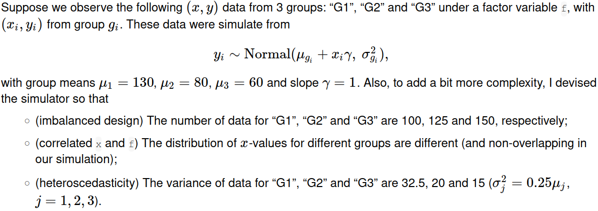
group.size <- c(100, 125, 150)
group.mean <- c(130, 80, 60)
group.variance <- 0.25 * group.mean
dat <- SimData(group.size, group.mean, group.variance)

ggplot(data = dat, mapping = aes(x = x, y = y, colour = f)) + geom_point()

​

​

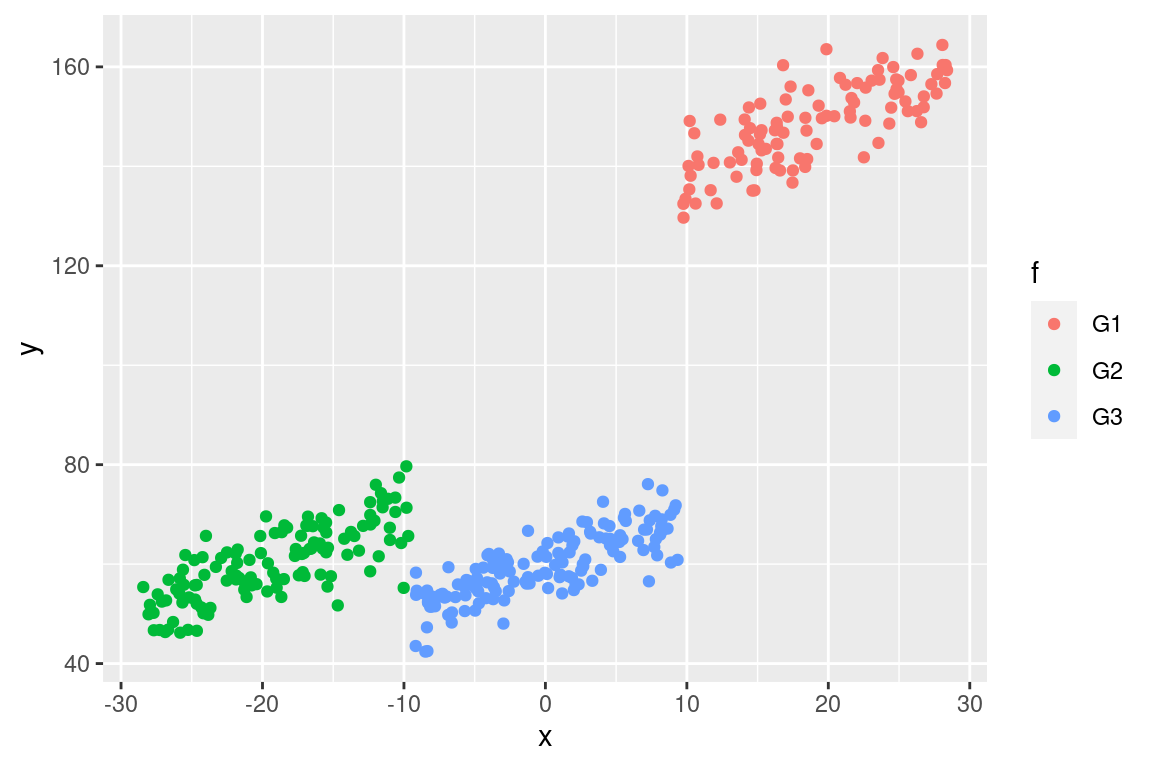
对每一组的均值和方差进行天真的计算是有误导性的，因为我们离事实很远！

## true values are 130, 80, 60
with(dat, tapply(y, f, mean))
##        G1        G2        G3 
## 148.36985  60.38273  59.45486

## true values are 32.5, 20 and 15
with(dat, tapply(y, f, var))
##       G1       G2       G3 
## 67.37108 55.25185 41.69867

对比编码

​

​

​

​

## treatment coding
contr.treatment(3)
##   2 3
## 1 0 0
## 2 1 0
## 3 0 1

## sum-to-zero coding
contr.sum(3)
##   [,1] [,2]
## 1    1    0
## 2    0    1
## 3   -1   -1

​

​

fit.treatment <- lm(y ~ f + x, dat, contrasts = list(f = "contr.treatment"))
coef(fit.treatment)
#(Intercept)         fG2         fG3           x 
#  128.94609   -48.71525   -69.03433     1.03121 

summary(fit.treatment)
anova(fit.treatment)

fit.sum <- lm(y ~ f + x, dat, contrasts = list(f = "contr.sum"))
coef(fit.sum)
#(Intercept)          f1          f2           x 
#  89.696234   39.249860   -9.465391    1.031210 

summary(fit.sum)
anova(fit.sum)

请注意，虽然使用不同的对比编码给出不同的回归系数，但它们实际上是等价的，产生相同的拟合值。

all.equal(fit.treatment$fitted.values, fit.sum$fitted.values)
## [1] TRUE

将群体均值与均数进行比较

​

​

​

​

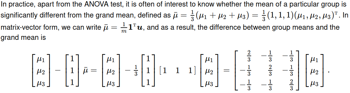
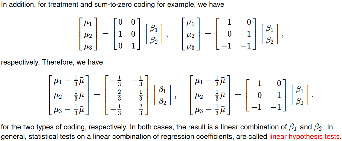
R中的线性假设检验

1.无花式包的香草方法()

​

​

## 3 x 2 linear combination matrix
wt.treatment <- matrix(c(-1, 2, -1, -1, -1, 2), nrow = 3) / 3
wt.sum <- matrix(c(1, 0, -1, 0, 1, -1), nrow = 3)

vanilla <- function (wt, beta.ind, lmfit) {
  ## beta coefficients and their covariance matrix
  beta <- coef(lmfit)[beta.ind]
  V <- vcov(lmfit)[beta.ind, beta.ind]
  ## linear combination and their standard errors
  MEAN <- c(wt %*% beta)
  ## get standard errors for sum of `LinearComb`
  SE <- sqrt(diag(wt %*% tcrossprod(V, wt)))
  ## perform t-test
  tscore <- MEAN / SE
  pvalue <- 2 * pt(abs(tscore), lmfit$df.residual, lower.tail = FALSE)
  ## return a matrix
  ans <- matrix(c(MEAN, SE, tscore, pvalue), ncol = 4L)
  colnames(ans) <- c("Estimate", "Std. Error", "t value", "Pr(>|t|)")
  printCoefmat(ans)
}

vanilla(wt.treatment, 2:3, fit.treatment)
##       Estimate Std. Error t value  Pr(>|t|)    
## [1,]  39.24986    0.90825  43.215 < 2.2e-16 ***
## [2,]  -9.46539    0.89404 -10.587 < 2.2e-16 ***
## [3,] -29.78447    0.32466 -91.741 < 2.2e-16 ***
## ---
## Signif. codes:  0 '***' 0.001 '**' 0.01 '*' 0.05 '.' 0.1 ' ' 1

vanilla(wt.sum, 2:3, fit.sum)  ## identical to above

2.使用包“multcomp”

​

​

## pad columns of zeros to zero out the effect of alpha and gamma
wt.treatment0 <- cbind(0, wt.treatment, 0)
wt.sum0 <- cbind(0, wt.sum, 0)

summary(glht(fit.treatment, linfct = wt.treatment0))
## Linear Hypotheses:
##        Estimate Std. Error t value Pr(>|t|)    
## 1 == 0  39.2499     0.9083   43.22   <2e-16 ***
## 2 == 0  -9.4654     0.8940  -10.59   <2e-16 ***
## 3 == 0 -29.7845     0.3247  -91.74   <2e-16 ***
## ---
## Signif. codes:  0 '***' 0.001 '**' 0.01 '*' 0.05 '.' 0.1 ' ' 1
## (Adjusted p values reported -- single-step method)

summary(glht(fit.sum, linfct = wt.sum0))  ## identical to above

3.使用软件包‘emmeans’

​

​

emmeans(fit.treatment, specs = eff ~ f)
## $emmeans
##  f  emmean    SE  df lower.CL upper.CL
##  G1  127.3 1.002 371    125.4    129.3
##  G2   78.6 0.874 371     76.9     80.3
##  G3   58.3 0.379 371     57.5     59.0
## 
## Confidence level used: 0.95 
## 
## $contrasts
##  contrast  estimate    SE  df t.ratio p.value
##  G1 effect    39.25 0.908 371  43.215  <.0001
##  G2 effect    -9.47 0.894 371 -10.587  <.0001
##  G3 effect   -29.78 0.325 371 -91.741  <.0001
## 
## P value adjustment: fdr method for 3 tests

emmeans(fit.sum, specs = eff ~ f)  ## identical to above

在这里，使用specs = ~f或specs = "f"，只报告$emmeans (边缘均值)组件。左手边的"eff“表示要调用eff.emmc()来应用对比，而$contrasts组件提供了这样的结果。

4.使用软件包“car”

linearHypothesis()函数来自cars，执行F-测试，以测试所有线性组合是否同时为0。因此，它不同于上面演示的t检验。此外，它还产生了错误：

linearHypothesis(fit.treatment, hypothesis.matrix = wt.treatment0)
#Error in solve.default(vcov.hyp) : 
#  system is computationally singular: reciprocal condition number = 1.12154e-17

linearHypothesis(fit.sum, hypothesis.matrix = wt.sum0)  ## identical to above

从某种意义上说，这个答案是我以前几个答案的总结。

• lm summary not display all factor levels

• How to set contrasts for my variable in regression analysis with R?

• Interpeting R significance codes for ANOVA table?

• Comparing all factor levels to the grand mean: can I tweak contrasts in linear model fitting to show all levels?

• Get p-value for group mean difference without refitting linear model with a new reference level

• How to conduct linear hypothesis test on regression coefficients with a clustered covariance matrix?