如何提高python非线性拟合的质量？

Question

我正在研究一个生化模型:有一种酶可以催化两次底物。通过命名：

*E=酶

*S=原始基板

*P=中间产物，它反过来是底物

*F=最终产品

我有这样的反应模式：

S+E <-> SE -> E+P <-> EP -> E+F

命名为A的第一催化反应和B的第二催化反应，我总共有6个动力学系数：

* ka = substrate+enzyme配合物(S +E -> SE)的形成

* kar =该配合物(SE -> S +E)的溶解(逆反应)

* kcata =催化系数(SE -> S+ P)

和类似的kb，kbr，kcatb

我还有两个实验数据集，其中记录了S、P和F三种物种的时间过程，但每种物种在不同的时间和不同的点数(每个样本的平均大小为12点)被取样。这两组对应于两种不同的初始酶浓度。然后我有两组二维数组，如S_E1t_i，concentration_t_i，P_E1t_i，concentration_t_i，F_E1t_i, concentration_t_i，以及类似的S_E2，P_E2，F_E2。获取时间的精度为1，在0-60,000 s范围内；例如，P_E1第一元素看起来类似于(t_i= 43280，conc.= 21.837)，但该范围内的测量是稀疏的。

我想对微分方程组进行动态拟合，以求出6个系数(各种k)的值，但我遇到了以下几个问题：

如果我设置

1. (0,600，1)，程序总是以“内存故障”崩溃，独立于我可以选择的求解器，即使Obj函数只在总共72个点上计算平方误差最小化；
2. 为了绕过这个问题，我重新离散了100 s间隔的时间；因此，报告实验浓度值，就像它们是在最接近的100整数s上实时获得的:这可能在拟合时产生错误，但我希望这是可以忽略不计的；然后，我声明m.time= np.linspace(0,600,101)，并相应地将所有数组映射到新的时间刻度；在这种情况下，
3. 只在使用APOPT或IPOPT求解器时才能工作(BPOPT总是返回“奇异矩阵”的错误)；然而，由于以下三个原因，所得到的拟合不太好(拟合点距离实验点很远)：

a.在拟合结束时，Obj函数非常大(> 10^3)，从而说明了实验值与拟合值之间的距离；

b.迭代次数仍低于最高阈值，因此增加该阈值的选择显然没有任何效果；

对初始条件的敏感性极高，因此拟合结果不可靠。

我试图设置一些选项来增加最大的迭代次数或类似的策略，但似乎没有任何效果。欢迎任何建议！

# -------------------- importing packages
import numpy as np
import matplotlib.pyplot as plt
from gekko import GEKKO


# -------------------- declaring functions 

def rediscr(myarr, delta): #rediscretizzation function
    mydarr = np.floor((myarr // delta)).astype(int)
    mydarr = mydarr * delta
    return mydarr


def rmap(mytim, mydatx, mydaty, indarr, selarr, concarr): #function to map the concentration values on the re-discretized times
    j=0
    for i in range(len(mytim)):
        if(mytim[i]==mydatx[j]):
            indarr = np.append(indarr, i).astype(int);      
            selarr[i] = 1
            concarr[i] = mydaty[j]
            j += 1
            if(j == len(mydatx)):
                break;
    return indarr

# -------------------- input data, plotting & rediscr.

SE1 = np.genfromtxt("s_e1.txt")
PE1 = np.genfromtxt("q_e1.txt")
FE1 = np.genfromtxt("p_e1.txt")

# dataset 2
SE2 = np.genfromtxt("s_e2.txt")
PE2 = np.genfromtxt("q_e2.txt")
FE2 = np.genfromtxt("p_e2.txt")

plt.plot(SE1[:,0],SE1[:,1],'ro', label="s_e1")
plt.plot(PE1[:,0],PE1[:,1],'bo', label="p_e1")
plt.plot(FE1[:,0],FE1[:,1],'go', label="f_e1")

# plt.plot(SE2[:,0],SE2[:,1],'ro', label="s_e2")
# plt.plot(PE2[:,0],PE2[:,1],'bo', label="p_e2")
# plt.plot(FE2[:,0],FE2[:,1],'go', label="f_e2")


step= 100  # rediscretization factor
nout= "2set6par100p" # prefix for the filename of output files

nST = rediscr(SE1[:,0], step)
nPT = rediscr(PE1[:,0], step)
nFT = rediscr(FE1[:,0], step) 

nST2 = rediscr(SE2[:,0], step)
nPT2 = rediscr(PE2[:,0], step)
nFT2 = rediscr(FE2[:,0], step) 



# start modeling with gekko
m = GEKKO(remote=False)

timestep= (60000 // step) +1
m.time = np.linspace(0,60000,timestep)

# definig indXX= array index of the positions corresponding to measured concentratio values; select_XX= boolean array =0 if there is no measure, =1 if the measure exists; conc_X= concentration value at the selected time
indST=np.array([]).astype(int)
indPT=np.array([]).astype(int)
indFT=np.array([]).astype(int)
select_s=np.zeros(len(m.time), dtype=int)
select_f=np.zeros(len(m.time), dtype=int)
select_p=np.zeros(len(m.time), dtype=int)
conc_s=np.zeros(len(m.time), dtype=float)
conc_f=np.zeros(len(m.time), dtype=float)
conc_p=np.zeros(len(m.time), dtype=float)

indST2=np.array([]).astype(int)
indFT2=np.array([]).astype(int)
indPT2=np.array([]).astype(int)
select_s2=np.zeros(len(m.time), dtype=int)
select_f2=np.zeros(len(m.time), dtype=int)
select_p2=np.zeros(len(m.time), dtype=int)
conc_s2=np.zeros(len(m.time), dtype=float)
conc_f2=np.zeros(len(m.time), dtype=float)
conc_p2=np.zeros(len(m.time), dtype=float)

indST= rmap(m.time, nST, SE1[:,1], indST, select_s, conc_s)
indPT= rmap(m.time, nPT, PE1[:,1], indPT, select_p, conc_p)
indFT= rmap(m.time, nFT, FE1[:,1], indFT, select_f, conc_f)

indST2= rmap(m.time, nST2, SE2[:,1], indST2, select_s2, conc_s2)
indPT2= rmap(m.time, nPT2, PE2[:,1], indPT2, select_p2, conc_p2)
indFT2= rmap(m.time, nFT2, FE2[:,1], indFT2, select_f2, conc_f2)


kenz1 = 0.000341; # value of a characteristic global constant of the first reaction (esperimentally determined)
kenz2 = 0.0000196; # value of a characteristic global constant of the first reaction (esperimentally determined)

ka = m.FV(value=0.001, lb=0); ka.STATUS = 1     #   parameter to change in fitting the curves
kar = m.FV(value=0.000018, lb=0); kar.STATUS = 1        # parameter to change in fitting the curves
kb = m.FV(value=0.000018, lb=0); kb.STATUS = 1         # parameter to change in fitting the curves
kbr = m.FV(value=0.00000005, lb=0); kbr.STATUS = 1        #  parameter to change in fitting the curves
kcata = m.FV(value=0.01, lb=0); kcata.STATUS = 1        #  parameter to change in fitting the curves
kcatb = m.FV(value=0.01, lb=0);  kcatb.STATUS = 1        #  parameter to change in fitting the curves



SC1 = m.Var(SE1[0,1], lb=0, ub=SE1[0,1]) # fit to measurement
FC1 = m.Var(0, lb=0, ub=SE1[0,1]) # fit to measurement
PC1 = m.Var(0, lb=0, ub=SE1[0,1])    # fit to measurement
E1 =m.Var(1, lb=0, ub=1) # for enzyme and enzymatic complexes, I have no experimental data
ES1=m.Var(0, lb=0, ub=1) # for enzyme and enzymatic complexes, I have no experimental data
EP1=m.Var(0, lb=0, ub=1) # for enzyme and enzymatic complexes, I have no experimental data
E2 =m.Var(2, lb=0, ub=2) # for enzyme and enzymatic complexes, I have no experimental data
ES2=m.Var(0, lb=0, ub=2) # for enzyme and enzymatic complexes, I have no experimental data
EP2=m.Var(0, lb=0, ub=2) # for enzyme and enzymatic complexes, I have no experimental data
SC2 = m.Var(SE2[0,1], lb=0, ub=SE2[0,1]) # fit to measurement
FC2 = m.Var(0, lb=0, ub=SE2[0,1]) # fit to measurement
PC2 = m.Var(0, lb=0, ub=SE2[0,1])    # fit to measurement

sels = m.Param(select_s) # boolean point in time for s species
selp = m.Param(select_p) # ""                        p
self = m.Param(select_f) # ""                        f 
c_s = m.Param(conc_s) # concentration values
c_p = m.Param(conc_p) # concentration values
c_f = m.Param(conc_f) # concentration values

sels2 = m.Param(select_s2) # boolean point in time for s species
selp2 = m.Param(select_p2) # ""                        p
self2 = m.Param(select_f2) # ""                        f 
c_s2 = m.Param(conc_s2) # concentration values
c_p2 = m.Param(conc_p2) # concentration values
c_f2 = m.Param(conc_f2) # concentration values

m.Equations([E1.dt() ==-ka * SC1 * E1 +(kar + kcata) * ES1 - kb * E1 * PC1 + (kbr + kcata) * EP1, \
PC1.dt() == kcata * ES1 - kb * E1 * PC1 +kbr * EP1, \
ES1.dt() == ka * E1 * SC1 - (kar + kcata) * ES1, \
SC1.dt() == -ka * SC1 * E1 + kar * ES1,\
EP1.dt() == kb * E1 * PC1 - (kbr + kcata) * EP1, \
FC1.dt() == kcata * EP1, \
E2.dt() == -ka * SC2 * E2 +(kar + kcatb) * ES2 - kb * E2 * PC2 + (kbr + kcatb) * EP2, \
PC2.dt() == kcatb * ES2 - kb * E2 * PC1 +kbr * EP2, \
ES2.dt() == ka * E2 * SC2 - (kar + kcatb) * ES2, \
SC2.dt() == -ka * SC2 * E2 + kar * ES2,\
EP2.dt() == kb * E2 * PC2 - (kbr + kcatb) * EP2, \
FC2.dt() == kcatb * EP2 ])

m.Minimize((sels*(SC1-c_s))**2 + (self*(FC1-c_f))**2 + (selp*(PC1-c_p))**2 + (sels2*(SC2-c_s2))**2 + (self2*(FC2-c_f2))**2 + (selp2*(PC2-c_p2))**2)

m.options.IMODE = 5   # dynamic estimation
m.options.SOLVER = 1
m.solve(disp=True, debug=False)    # display solver output
ai= m.options.APPINFO

if(ai):
    print("Impossibile to solve!\n")
else: # output datafiles and graphs
    fk_enz_a = kcata.value[0] /((kar.value[0] + kcata.value[0])/ka.value[0])
    fk_enz_b = kcatb.value[0] /((kbr.value[0] + kcatb.value[0])/kb.value[0])
    frac_kenza = fk_enz_a/kenz1
    frac_kenzb = fk_enz_b/kenz2
    print("Solver APOPT - ka= ", ka.value[0], "kb= ",kb.value[0], "kar= ", kar.value[0], "kbr= ", kbr.value[0], "kcata= ", kcata.value[0], "kcata= ", kcatb.value[0], "kenz_a= ", fk_enz_a, "frac_kenz_a=", frac_kenza, "kenz_b= ", fk_enz_b, "frac_kenz_b=", frac_kenzb)     

    solv="_a_";
    tis=m.time[indST]
    fcs=np.array(SC1)
    pfcs= fcs[indST]
    tif=m.time[indFT]
    fcf=np.array(FC1)
    pfcf=fcf[indFT]
    tip=m.time[indPT]
    fcp=np.array(PC1)
    pfcp=fcp[indPT]
    fce=np.array(E1)
    fces=np.array(ES1)
    fcep=np.array(EP1)

    np.savetxt(nout+solv+"_fit1.txt", np.c_[m.time, fcs, fcp, fcf, fce, fces, fcep], fmt='%f', delimiter='\t')
    np.savetxt(nout+solv+"_s1.txt", np.c_[tis, pfcs], fmt='%f', delimiter='\t')
    np.savetxt(nout+solv+"_p1.txt", np.c_[tip, pfcp], fmt='%f', delimiter='\t')
    np.savetxt(nout+solv+"_f1.txt", np.c_[tif, pfcf], fmt='%f', delimiter='\t')


    tis2=m.time[indST2]
    fcs2=np.array(SC2)
    pfcs2= fcs2[indST2]
    tif2=m.time[indFT2]
    fcf2=np.array(FC2)
    pfcf2=fcf2[indFT2]
    tip2=m.time[indPT2]
    fcp2=np.array(PC2)
    pfcp2=fcp2[indPT2]
    fce2=np.array(E2)
    fces2=np.array(ES2)
    fcep2=np.array(EP2)

    np.savetxt(nout+solv+"_fit2.txt", np.c_[m.time, fcs2, fcp2, fcf2, fce2, fces2, fcep2], fmt='%f', delimiter='\t')
    np.savetxt(nout+solv+"_s2.txt", np.c_[tis2, pfcs2], fmt='%f', delimiter='\t')
    np.savetxt(nout+solv+"_p2.txt", np.c_[tip2, pfcp2], fmt='%f', delimiter='\t')
    np.savetxt(nout+solv+"_f2.txt", np.c_[tif2, pfcf2], fmt='%f', delimiter='\t')


    plt.plot(tis, pfcs,'gx', label="Fs_e1")
    plt.plot(tip, pfcp,'bx', label="Fp_e1")
    plt.plot(tif, pfcf,'rx', label="Ff_e1")

    plt.plot(tis2, pfcs2,'gx', label="Fs_e2")
    plt.plot(tip2, pfcp2,'bx', label="Fp_e2")
    plt.plot(tif2, pfcf2,'rx', label="Ff_e2")



    plt.axis([0, 60000, 0, 60])
    plt.legend()
    plt.savefig(nout+solv+"fit.png")

    plt.close()

Answer 1

这里没有s_e1.txt或其他数据文件，因此我将给出一个示例问题，说明您可以使用的一些方法。不过，让我就你的问题给你一些深刻的见解：

• 与m.time=np.linspace(0,60000,1)的错误是只有1时间点，这会产生数组array([0.])。对于动态问题，比如array([ 0., 60000.]).
• If，至少需要两个时间点才能给出np.linspace(0,60000,2)，您有太多的时间点，比如np.linspace(0,1,60000)，那么应用程序就会耗尽内存，因为如果您使用本地32位remote=False应用程序，那么问题太大了(>4 GB)。对于编译为64位executables.
• You的Linux或MacOS版本来说，这不应该是一个问题，因为这些版本可以包括您的测量发生的确切时间点。没有必要给出大致的时间点。您可以设置m.time = [0,0.1,0.5,0.9,...,50000,60000]。
• 设置了一个目标，如果缺少特定的时间点，就跳过它们。下面的最小示例演示了当p1或p2为零时如何跳过度量。对斜率a和b进行了估算。忽略了-5在m1中的值和-6在m2中的值。

​

​

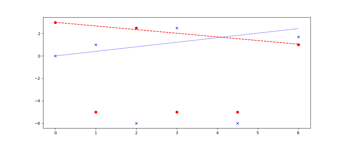
from gekko import GEKKO
m = GEKKO()
m.time = [0,1,2,3,4.5,6]
a = m.FV(); a.STATUS = 1
b = m.FV(); b.STATUS = 1
p1 = m.Param([0,0,1,0,0,1]) # indicate where there are measurements
p2 = m.Param([1,1,0,1,0,1])
m1 = m.Param([3,-5,2.5,-5,-5,1.0]) # measurements
m2 = m.Param([0,1,-6,2.5,-6,1.7])
v1 = m.Var(m1) # initialize with measurements
v2 = m.Var(m2)
# add equations
m.Equations([v1.dt()==a, v2.dt()==b])
# add objective function
m.Minimize(p1*(m1-v1)**2)
m.Minimize(p2*(m2-v2)**2)
m.options.IMODE = 6
m.solve()

import matplotlib.pyplot as plt
plt.figure(figsize=(12,5))
plt.plot(m.time,v1,'r--',label='v1')
plt.plot(m.time,v2,'b:',label='v2')
plt.plot(m.time,m1,'ro',label='m1')
plt.plot(m.time,m2,'bx',label='m2')
plt.savefig('demo.png'); plt.show()