图解预测概率(logit)

Question

目前，我正试图在r中绘制logit模型的预测概率。我遵循了这个链接的方法：https://stats.idre.ucla.edu/r/dae/logit-regression/。

考虑到利益集团类型，我已经成功地为布鲁塞尔办事处制作了地块。不过，我只想描绘个别的影响:例如，我想绘制布鲁塞尔办事处在与欧洲议会议员举行会议时的预测概率(即，当你有布鲁塞尔办事处时，与欧洲议会议员会晤的可能性是多少？)此外，我希望看到员工规模和/或组织形式对因变量的影响。

我还没有找到这样的办法。有什么建议吗？

提前谢谢你。

我的变量：

与欧洲议会议员的会议(因变量，虚拟)1是0否

利益集团类型(分类)1企业2咨询3非政府组织4公共当局5机构6工会/prof.org。7其他

布鲁塞尔办事处1是0否

组织形式1个人组织。2国家协会3欧洲协会4其他

工作人员人数(计数变量，以全时等值表示)范围为0.25至40

Answer 1

从昨天开始。

library(ggplot2)

# mydata <- read.csv("binary.csv")
str(mydata)
#> 'data.frame':    400 obs. of  4 variables:
#>  $ admit: int  0 1 1 1 0 1 1 0 1 0 ...
#>  $ gre  : int  380 660 800 640 520 760 560 400 540 700 ...
#>  $ gpa  : num  3.61 3.67 4 3.19 2.93 3 2.98 3.08 3.39 3.92 ...
#>  $ rank : int  3 3 1 4 4 2 1 2 3 2 ...

mydata$rank <- factor(mydata$rank)

mylogit <- glm(admit ~ gre + gpa + rank, data = mydata, family = "binomial")

summary(mylogit)
#> 
#> Call:
#> glm(formula = admit ~ gre + gpa + rank, family = "binomial", 
#>     data = mydata)
#> 
#> Deviance Residuals: 
#>     Min       1Q   Median       3Q      Max  
#> -1.6268  -0.8662  -0.6388   1.1490   2.0790  
#> 
#> Coefficients:
#>              Estimate Std. Error z value Pr(>|z|)    
#> (Intercept) -3.989979   1.139951  -3.500 0.000465 ***
#> gre          0.002264   0.001094   2.070 0.038465 *  
#> gpa          0.804038   0.331819   2.423 0.015388 *  
#> rank2       -0.675443   0.316490  -2.134 0.032829 *  
#> rank3       -1.340204   0.345306  -3.881 0.000104 ***
#> rank4       -1.551464   0.417832  -3.713 0.000205 ***
#> ---
#> Signif. codes:  0 '***' 0.001 '**' 0.01 '*' 0.05 '.' 0.1 ' ' 1
#> 
#> (Dispersion parameter for binomial family taken to be 1)
#> 
#>     Null deviance: 499.98  on 399  degrees of freedom
#> Residual deviance: 458.52  on 394  degrees of freedom
#> AIC: 470.52
#> 
#> Number of Fisher Scoring iterations: 4

我们将在x轴上绘制GPA图，让我们生成一些点

range(mydata$gpa) # using GPA for your staff size
#> [1] 2.26 4.00

gpa_sequence <- seq(from = 2.25, to = 4.01, by = .01) # 177 points along x axis

这是在IDRE的例子，但他们使它变得复杂。第一步构建一个数据框架，其中包含我们的GPA点序列，该列中每个条目的GRE平均值，以及我们的4个因素重复了177次。

constantGRE <- with(mydata, data.frame(gre = mean(gre), # keep GRE constant
                                       gpa = rep(gpa_sequence, each = 4), # once per factor level
                                       rank = factor(rep(1:4, times = 177)))) # there's 177

str(constantGRE)
#> 'data.frame':    708 obs. of  3 variables:
#>  $ gre : num  588 588 588 588 588 ...
#>  $ gpa : num  2.25 2.25 2.25 2.25 2.26 2.26 2.26 2.26 2.27 2.27 ...
#>  $ rank: Factor w/ 4 levels "1","2","3","4": 1 2 3 4 1 2 3 4 1 2 ...

对177个GPA值*4个因子水平中的每一个进行预测。将该预测放入一个名为theprediction的新列中

constantGRE$theprediction <- predict(object = mylogit, 
                                      newdata = constantGRE, 
                                      type = "response")

绘制每等级一条线，为线条涂上唯一的颜色。这些线不是直的，也不是完全平行的，也不是等距的。

ggplot(constantGRE, aes(x = gpa, y = theprediction, color = rank)) +
  geom_smooth()
#> `geom_smooth()` using method = 'loess' and formula 'y ~ x'

​

​

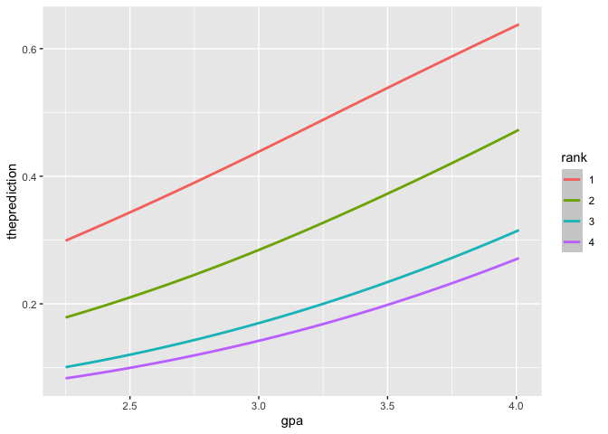
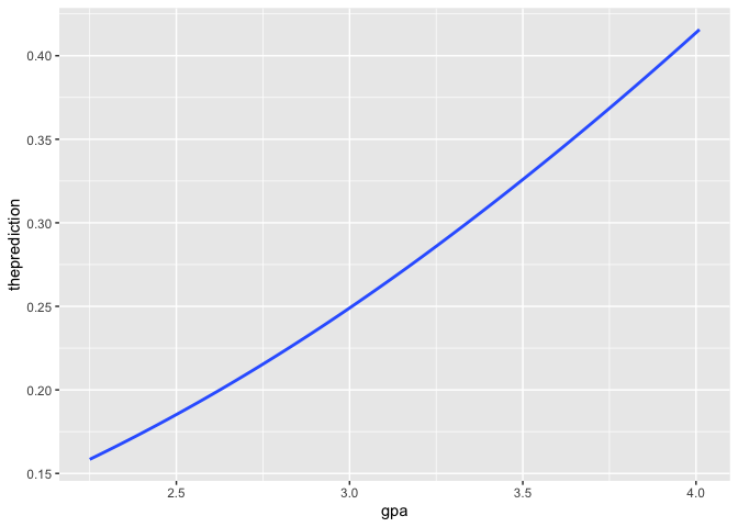
你可能会被诱惑，只是average的台词。不要。如果你想知道GPA的GRE，不包括排名，建立一个新的模型，因为(0.6357521 + 0.4704174 + 0.3136242 + 0.2700262) / 4不是正确的答案。

那，我们做吧。

# leave rank out call it new name

mylogit2 <- glm(admit ~ gre + gpa, data = mydata, family = "binomial")
summary(mylogit2)
#> 
#> Call:
#> glm(formula = admit ~ gre + gpa, family = "binomial", data = mydata)
#> 
#> Deviance Residuals: 
#>     Min       1Q   Median       3Q      Max  
#> -1.2730  -0.8988  -0.7206   1.3013   2.0620  
#> 
#> Coefficients:
#>              Estimate Std. Error z value Pr(>|z|)    
#> (Intercept) -4.949378   1.075093  -4.604 4.15e-06 ***
#> gre          0.002691   0.001057   2.544   0.0109 *  
#> gpa          0.754687   0.319586   2.361   0.0182 *  
#> ---
#> Signif. codes:  0 '***' 0.001 '**' 0.01 '*' 0.05 '.' 0.1 ' ' 1
#> 
#> (Dispersion parameter for binomial family taken to be 1)
#> 
#>     Null deviance: 499.98  on 399  degrees of freedom
#> Residual deviance: 480.34  on 397  degrees of freedom
#> AIC: 486.34
#> 
#> Number of Fisher Scoring iterations: 4

重复该过程的其余部分以获得一行

constantGRE2 <- with(mydata, data.frame(gre = mean(gre),
                                       gpa = gpa_sequence))
constantGRE2$theprediction <- predict(object = mylogit2, 
                                      newdata = constantGRE2, 
                                      type = "response")
ggplot(constantGRE2, aes(x = gpa, y = theprediction)) +
  geom_smooth()
#> `geom_smooth()` using method = 'loess' and formula 'y ~ x'

​

​

Answer 2

由于您没有提供数据，所以我将使用您熟悉的UCLA示例中的dataset。你想这么做吗(假设排名是你的变量之一).

library(ggplot2)

mydata <- read.csv("binary.csv")
mydata$rank <- factor(mydata$rank)

mylogit <- glm(admit ~ gre + gpa + rank, data = mydata, family = "binomial")
summary(mylogit)
#> 
#> Call:
#> glm(formula = admit ~ gre + gpa + rank, family = "binomial", 
#>     data = mydata)
#> 
#> Deviance Residuals: 
#>     Min       1Q   Median       3Q      Max  
#> -1.6268  -0.8662  -0.6388   1.1490   2.0790  
#> 
#> Coefficients:
#>              Estimate Std. Error z value Pr(>|z|)    
#> (Intercept) -3.989979   1.139951  -3.500 0.000465 ***
#> gre          0.002264   0.001094   2.070 0.038465 *  
#> gpa          0.804038   0.331819   2.423 0.015388 *  
#> rank2       -0.675443   0.316490  -2.134 0.032829 *  
#> rank3       -1.340204   0.345306  -3.881 0.000104 ***
#> rank4       -1.551464   0.417832  -3.713 0.000205 ***
#> ---
#> Signif. codes:  0 '***' 0.001 '**' 0.01 '*' 0.05 '.' 0.1 ' ' 1
#> 
#> (Dispersion parameter for binomial family taken to be 1)
#> 
#>     Null deviance: 499.98  on 399  degrees of freedom
#> Residual deviance: 458.52  on 394  degrees of freedom
#> AIC: 470.52
#> 
#> Number of Fisher Scoring iterations: 4

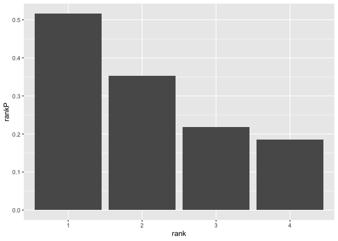
newdata1 <- with(mydata, data.frame(gre = mean(gre), gpa = mean(gpa), rank = factor(1:4)))

newdata1
#>     gre    gpa rank
#> 1 587.7 3.3899    1
#> 2 587.7 3.3899    2
#> 3 587.7 3.3899    3
#> 4 587.7 3.3899    4

newdata1$rankP <- predict(mylogit, newdata = newdata1, type = "response")
newdata1
#>     gre    gpa rank     rankP
#> 1 587.7 3.3899    1 0.5166016
#> 2 587.7 3.3899    2 0.3522846
#> 3 587.7 3.3899    3 0.2186120
#> 4 587.7 3.3899    4 0.1846684

ggplot(newdata1, aes(x = rank, y = rankP)) +
   geom_col()

​

​