单周期傅里叶窗优化我的代码效率很低

Question

日安

编辑：什么我想：从任何电流/电压波形的电力系统(PS)，我希望滤波50赫兹(基本)均方根值的幅度(和有效的角度)。测量的电流包含100 as到1250 as之间的所有谐波，这取决于设备。不能用带有这些谐波的波来分析和计算，你的误差会变得如此之大(取决于设备)，以至于PS保护设备计算不正确的数量。附加的信号还涉及许多其他频率分量。

My aim：PS保护继电器是特殊的，在很短的时间内计算一个20 PS的窗口。我不想弄到手。我正在使用外部记录技术和测试继电器所看到的是真实的，他们正确的操作。因此，我需要做他们所做的，只保留50赫兹的数值，没有任何谐波和直流。

重要的预期结果：给定信号中的任何频率分量，我想看到任意给定谐波的幅度(基波的150,250-3次谐波和5次谐波)以及直流的幅度。这将告诉我什么类型的PS设备可能注入这些频率。重要的是，我提供的频率和答案是一个向量的频率，只有与所有其他值过滤出来。基本的RMS与RMS不同，其因数为4000 A(仅50 of )和4500 A(包括其他频率)。

此代码计算给定频率的一个周期Fourier值(RMS)。有时我想叫傅里叶滤波器？用于电力系统50 0Hz/0HZ/150 0Hz模拟分析。(答案经过测试，是正确的基本均方根值。(https://users.wpi.edu/~goulet/Matlab/overlap/trigfs.html)

对于一个大的示例来说，代码非常慢。对于55000个数据点，它需要12秒。对于3个电压和3个电流，这是非常缓慢的。我每天看1000多张唱片。

我该如何增强它？有哪些Python技巧和技巧/库可以附加到我的列表/数组中。(也可以随意重写或使用代码)。我使用代码在给定的时间从信号中提取某些值。(这就像读取电力系统分析专用程序中的值一样)编辑:通过加载和使用文件，代码可以粘贴它：

import matplotlib.pyplot as plt
import csv
import math
import numpy as np
import cmath

# FILES ATTACHED TO POST
filenamecfg = r"E:/Python_Practise/2019-10-21 13-54-38-482.CFG"
filename = r"E:/Python_Practise/2019-10-21 13-54-38-482.DAT"

t = []
IR = []
newIR=[]
with open(filenamecfg,'r') as csvfile1:
    cfgfile = [row for row in csv.reader(csvfile1, delimiter=',')]
    numberofchannels=int(np.array(cfgfile)[1][0])
    scaleval = float(np.array(cfgfile)[3][5])
    scalevalI = float(np.array(cfgfile)[8][5])
    samplingfreq = float(np.array(cfgfile)[numberofchannels+4][0])
    numsamples = int(np.array(cfgfile)[numberofchannels+4][1])
    freq = float(np.array(cfgfile)[numberofchannels+2][0])
    intsample = int(samplingfreq/freq)
    #TODO neeeed to get number of samples and frequency and detect 
#automatically
    #scaleval = np.array(cfgfile)[3]
    print('multiplier:',scaleval)
    print('SampFrq:',samplingfreq)
    print('NumSamples:',numsamples)
    print('Freq:',freq)


with open(filename,'r') as csvfile:
    plots = csv.reader(csvfile, delimiter=',')
    for row in plots:
        t.append(float(row[1])/1000000) #get time from us to s
        IR.append(float(row[6]))

newIR = np.array(IR) * scalevalI
t = np.array(t)


def mag_and_theta_for_given_freq(f,IVsignal,Tsignal,samples): #samples are the sample window size you want to caclulate for (256 in my case)
    # f in hertz, IVsignal, Tsignal in numpy.array
    timegap = Tsignal[2]-Tsignal[3]
    pi = math.pi
    w = 2*pi*f
    Xr = []
    Xc = []
    Cplx = []
    mag = []
    theta = []
    #print("Calculating for frequency:",f)
    for i in range(len(IVsignal)-samples): 
        newspan = range(i,i+samples)
        timewindow = Tsignal[newspan]
        #print("this is my time: ",timewindow)
        Sig20ms = IVsignal[newspan]
        N = len(Sig20ms) #get number of samples of my current Freq
        RealI = np.multiply(Sig20ms, np.cos(w*timewindow)) #Get Real and Imaginary part of any signal for given frequency
        ImagI = -1*np.multiply(Sig20ms, np.sin(w*timewindow)) #Filters and calculates 1 WINDOW RMS (root mean square value).
        #calculate for whole signal and create a new vector. This is the RMS vector (used everywhere in power system analysis)
        Xr.append((math.sqrt(2)/N)*sum(RealI)) ### TAKES SO MUCH TIME
        Xc.append((math.sqrt(2)/N)*sum(ImagI)) ## these steps make RMS
        Cplx.append(complex(Xr[i],Xc[i]))
        mag.append(abs(Cplx[i]))
        theta.append(np.angle(Cplx[i]))#th*180/pi # this can be used to get Degrees if necessary
        #also for freq 0 (DC) id the offset is negative how do I return a negative to indicate this when i'm using MAGnitude or Absolute value
    return Cplx,mag,theta #mag[:,1]#,theta # BUT THE MAGNITUDE WILL NEVER BE zero

myZ,magn,th = mag_and_theta_for_given_freq(freq,newIR,t,intsample)

plt.plot(newIR[0:30000],'b',linewidth=0.4)#, label='CFG has been loaded!')
plt.plot(magn[0:30000],'r',linewidth=1)

plt.show()

考虑到附加的文件，粘贴的代码运行平稳。

编辑:请在这里找到一个测试CSV文件和COMTRADE测试文件: CSV：MtYAeTBm7tNQTcQkTnFWQ4LUu

商品贸易委员会( COMTRADE Ocv9x/view?usp=共享 A9GrqAgFtD/view?usp=共享 )

Answer 1

前言

正如我在之前的评论中所说：

您的代码主要依赖于具有大量指数化和标量操作的for循环。您已经导入了numpy，因此您应该利用矢量化。

这个答案是你的解决方案的开始。

轻量化MCVE

首先，我们为MCVE创建了一个试用信号：

import numpy as np

# Synthetic signal sampler: 5s sampled as 400 Hz
fs = 400 # Hz
t = 5    # s
t = np.linspace(0, t, fs*t+1)

# Synthetic Signal: Amplitude is about 325V @50Hz
A = 325 # V
f = 50  # Hz
y = A*np.sin(2*f*np.pi*t) # V

然后，我们可以使用通常的公式计算这个信号的均方根：

# Actual definition of RMS:
yrms = np.sqrt(np.mean(y**2)) # 229.75 V

或者，我们也可以使用DFT (在numpy.fft中实现为rfft )计算它：

# RMS using FFT:
Y = np.fft.rfft(y)/y.size
Yrms = np.sqrt(np.real(Y[0]**2 + np.sum(Y[1:]*np.conj(Y[1:]))/2)) # 229.64 V

这里可以找到最后一个公式起作用的原因的演示。这是有效的，因为Parseval定理暗示傅里叶变换确实节省能量。

这两个版本都使用了矢量化函数，不需要分割实部和虚部进行计算，然后重新组装成一个复数。

MCVE:窗口

我怀疑您希望将此功能作为一个长期意甲的窗口，在这里RMS值即将发生变化。然后，我们可以使用提供时间序列商品的pandas库来解决这个问题。

import pandas as pd

我们封装了RMS功能：

def rms(y):
    Y = 2*np.fft.rfft(y)/y.size
    return np.sqrt(np.real(Y[0]**2 + np.sum(Y[1:]*np.conj(Y[1:]))/2))

我们产生一个阻尼信号(可变均方根)

y = np.exp(-0.1*t)*A*np.sin(2*f*np.pi*t) 

为了利用rolling或resample方法，我们将试用信号封装到数据文件中：

df = pd.DataFrame(y, index=t*pd.Timedelta('1s'), columns=['signal'])

你的信号的滚动均方根是：

df['rms'] = df.rolling(int(fs/f)).agg(rms)

定期抽样的均方根是：

df['signal'].resample('1s').agg(rms)

后一批返回：

00:00:00    2.187840e+02
00:00:01    1.979639e+02
00:00:02    1.791252e+02
00:00:03    1.620792e+02
00:00:04    1.466553e+02

信号调理

满足您只保留基本谐波(50 Hz)的需要，一个简单的解决方案可以是线性下降趋势 (消除常数和线性趋势)，然后是一个巴特沃斯 过滤器 (带通滤波器)。

我们用其他频率和线性趋势产生合成信号：

y = np.exp(-0.1*t)*A*(np.sin(2*f*np.pi*t) \
     + 0.2*np.sin(8*f*np.pi*t) + 0.1*np.sin(16*f*np.pi*t)) \
     + A/20*t + A/100

然后我们给信号设定条件：

from scipy import signal
yd = signal.detrend(y, type='linear')
filt = signal.butter(5, [40,60], btype='band', fs=fs, output='sos', analog=False)
yfilt = signal.sosfilt(filt, yd)

从图形上看，它导致：

​

​

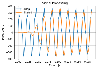
在均方根计算前恢复信号调理。