适用于小信号模型的pyhf收敛失效拟合

Question

(这是我们( pyhf团队)最近遇到的一个问题，我们认为这个问题很好，值得分享。所以我们在这里发布了一个修改过的版本。

我试着用pyhf v0.4.0做一个简单的假设检验。我正在使用的模型有一个小的信号，所以我需要扫描信号强度几乎所有的出路到mu=100。然而，我一直有一个收敛问题。为什么适配不能收敛？

下面是我的环境、我正在使用的代码以及我的错误。

环境

$ "$(which python3)" --version
Python 3.7.5
$ python3 -m venv "${HOME}/.venvs/example"
$ . "${HOME}/.venvs/example/bin/activate"

(example) $ python -m pip install --upgrade pip setuptools wheel
(example) $ cat requirements.txt
pyhf~=0.4.0
black
(example) $ python -m pip install -r requirements.txt
(example) $ pip list
Package            Version
------------------ --------
appdirs            1.4.3   
attrs              19.3.0  
black              19.10b0
Click              7.0     
importlib-metadata 1.5.0   
jsonpatch          1.25    
jsonpointer        2.0     
jsonschema         3.2.0   
numpy              1.18.1  
pathspec           0.7.0   
pip                20.0.2  
pkg-resources      0.0.0   
pyhf               0.4.0   
pyrsistent         0.15.7  
PyYAML             5.3     
regex              2020.1.8
scipy              1.4.1   
setuptools         45.1.0  
six                1.14.0  
toml               0.10.0  
tqdm               4.42.1  
typed-ast          1.4.1   
wheel              0.34.2  
zipp               2.1.0

代码

# example.py
import pyhf
from pyhf import Model, infer


def main():
    signal=[0.00000000e+00,2.16147594e-04,4.26391320e-04,8.53157029e-04,
            7.95947245e-04,1.85458682e-03,3.15515589e-03,4.22895664e-03,
            4.65887617e-03,7.35380863e-03,8.71947686e-03,7.94697901e-03,
            1.02721341e-02,9.24346489e-03,9.38926633e-03,9.68742497e-03,
            8.11072856e-03,7.71003446e-03,6.80873211e-03,5.43234586e-03,
            4.98376829e-03,4.72218222e-03,3.40645378e-03,3.44950579e-03,
            2.61473009e-03,2.18345641e-03,2.00960464e-03,1.33786215e-03,
            1.18440675e-03,8.36366201e-04,5.99855228e-04,4.27406780e-04,
            2.71607026e-04,1.81370902e-04,1.03710513e-04,4.42737056e-05,
            2.25835175e-05,1.04470885e-05,4.08162922e-06,3.20004812e-06,
            3.37990384e-07,6.72843977e-07,0.00000000e+00,9.08675772e-08,
            0.00000000e+00]

    bkgrd=[1.47142981e+03,9.07095061e+02,9.11188195e+02,7.06123452e+02,
           6.08054685e+02,5.23577562e+02,4.41672633e+02,4.00423307e+02,
           3.59576067e+02,3.26368076e+02,2.88077216e+02,2.48887339e+02,
           2.20355981e+02,1.91623853e+02,1.57733823e+02,1.32733279e+02,
           1.12789438e+02,9.53141118e+01,8.15735557e+01,6.89604141e+01,
           5.64245978e+01,4.49094779e+01,3.95547919e+01,3.13005748e+01,
           2.55212288e+01,1.93057913e+01,1.48268648e+01,1.13639821e+01,
           8.64408136e+00,5.81608649e+00,3.98839138e+00,2.61636610e+00,
           1.55906281e+00,1.08550560e+00,5.57450828e-01,2.25258250e-01,
           2.05230728e-01,1.28735312e-01,6.13798028e-02,2.00805073e-02,
           5.91436617e-02,0.00000000e+00,0.00000000e+00,0.00000000e+00,
           0.00000000e+00]

    spec = {
        "channels": [
            {
                "name": "singlechannel",
                "samples": [
                    {
                        "name": "signal",
                        "data": signal,
                        "modifiers": [
                            {"name": "mu", "type": "normfactor", "data": None}
                        ],
                    },
                    {"name": "background", "data": bkgrd, "modifiers": [],},
                ],
            }
        ]
    }

    model = pyhf.Model(spec)
    hypo_tests = pyhf.infer.hypotest(
        1.0,
        model.expected_data([0]),
        model,
        0.5,
        [(0, 80)],
        return_expected_set=True,
        return_test_statistics=True,
        qtilde=True,
    )
    print(hypo_tests)


if __name__ == "__main__":
    main()

错误

(example) $ python example.py
/home/jovyan/.venvs/example/lib/python3.7/site-packages/pyhf/tensor/numpy_backend.py:253: RuntimeWarning: divide by zero encountered in log
  return n * np.log(lam) - lam - gammaln(n + 1.0)
/home/jovyan/.venvs/example/lib/python3.7/site-packages/pyhf/tensor/numpy_backend.py:253: RuntimeWarning: invalid value encountered in multiply
  return n * np.log(lam) - lam - gammaln(n + 1.0)
ERROR:pyhf.optimize.opt_scipy:     fun: nan
     jac: array([nan])
 message: 'Iteration limit exceeded'
    nfev: 1300003
     nit: 100001
    njev: 100001
  status: 9
 success: False
       x: array([0.499995])
Traceback (most recent call last):
  File "example.py", line 65, in <module>
    main()
  File "example.py", line 59, in main
    qtilde=True,
  File "/home/jovyan/.venvs/example/lib/python3.7/site-packages/pyhf/infer/__init__.py", line 82, in hypotest
    asimov_data = generate_asimov_data(asimov_mu, data, pdf, init_pars, par_bounds)
  File "/home/jovyan/.venvs/example/lib/python3.7/site-packages/pyhf/infer/utils.py", line 8, in generate_asimov_data
    bestfit_nuisance_asimov = fixed_poi_fit(asimov_mu, data, pdf, init_pars, par_bounds)
  File "/home/jovyan/.venvs/example/lib/python3.7/site-packages/pyhf/infer/mle.py", line 62, in fixed_poi_fit
    **kwargs,
  File "/home/jovyan/.venvs/example/lib/python3.7/site-packages/pyhf/optimize/opt_scipy.py", line 47, in minimize
    assert result.success
AssertionError

Answer 1

从模型的角度来看，背景估计不应该是零，所以在模型中添加一个1e-7的epsilon，然后添加1%的背景不确定性。虽然这里的问题是信号强度的合理间隔在μ ∈ [0,10]之间。如果你的模型是这样的，你对这个范围内的信号强度不敏感，那么你应该测试一个新的信号模型，它是由某个尺度因子缩放的原始信号。

环境

为了便于可视化，让我们对环境进行一些扩展

(example) $ cat requirements.txt 
pyhf~=0.4.0
black
matplotlib~=3.1
altair~=4.0

代码

# answer.py
import pyhf
from pyhf import Model, infer
import numpy as np
import matplotlib.pyplot as plt
import pyhf.contrib.viz.brazil


def invert_interval(test_mus, hypo_tests, test_size=0.05):
    cls_obs = np.array([test[0] for test in hypo_tests]).flatten()
    cls_exp = [
        np.array([test[1][i] for test in hypo_tests]).flatten() for i in range(5)
    ]
    crossing_test_stats = {"exp": [], "obs": None}
    for cls_exp_sigma in cls_exp:
        crossing_test_stats["exp"].append(
            np.interp(
                test_size, list(reversed(cls_exp_sigma)), list(reversed(test_mus))
            )
        )
    crossing_test_stats["obs"] = np.interp(
        test_size, list(reversed(cls_obs)), list(reversed(test_mus))
    )
    return crossing_test_stats


def main():
    unscaled_signal=[0.00000000e+00,2.16147594e-04,4.26391320e-04,8.53157029e-04,
                     7.95947245e-04,1.85458682e-03,3.15515589e-03,4.22895664e-03,
                     4.65887617e-03,7.35380863e-03,8.71947686e-03,7.94697901e-03,
                     1.02721341e-02,9.24346489e-03,9.38926633e-03,9.68742497e-03,
                     8.11072856e-03,7.71003446e-03,6.80873211e-03,5.43234586e-03,
                     4.98376829e-03,4.72218222e-03,3.40645378e-03,3.44950579e-03,
                     2.61473009e-03,2.18345641e-03,2.00960464e-03,1.33786215e-03,
                     1.18440675e-03,8.36366201e-04,5.99855228e-04,4.27406780e-04,
                     2.71607026e-04,1.81370902e-04,1.03710513e-04,4.42737056e-05,
                     2.25835175e-05,1.04470885e-05,4.08162922e-06,3.20004812e-06,
                     3.37990384e-07,6.72843977e-07,0.00000000e+00,9.08675772e-08,
                     0.00000000e+00]

    bkgrd=[1.47142981e+03,9.07095061e+02,9.11188195e+02,7.06123452e+02,
           6.08054685e+02,5.23577562e+02,4.41672633e+02,4.00423307e+02,
           3.59576067e+02,3.26368076e+02,2.88077216e+02,2.48887339e+02,
           2.20355981e+02,1.91623853e+02,1.57733823e+02,1.32733279e+02,
           1.12789438e+02,9.53141118e+01,8.15735557e+01,6.89604141e+01,
           5.64245978e+01,4.49094779e+01,3.95547919e+01,3.13005748e+01,
           2.55212288e+01,1.93057913e+01,1.48268648e+01,1.13639821e+01,
           8.64408136e+00,5.81608649e+00,3.98839138e+00,2.61636610e+00,
           1.55906281e+00,1.08550560e+00,5.57450828e-01,2.25258250e-01,
           2.05230728e-01,1.28735312e-01,6.13798028e-02,2.00805073e-02,
           5.91436617e-02,0.00000000e+00,0.00000000e+00,0.00000000e+00,
           0.00000000e+00]

    scale_factor = 500
    signal = np.asarray(unscaled_signal) * scale_factor
    epsilon = 1e-7
    background = np.asarray(bkgrd) + epsilon

    spec = {
        "channels": [
            {
                "name": "singlechannel",
                "samples": [
                    {
                        "name": "signal",
                        "data": signal.tolist(),
                        "modifiers": [
                            {"name": "mu", "type": "normfactor", "data": None}
                        ],
                    },
                    {
                        "name": "background",
                        "data": background.tolist(),
                        "modifiers": [
                            {
                                "name": "uncert",
                                "type": "shapesys",
                                "data": (0.01 * background).tolist(),
                            },
                        ],
                    },
                ],
            }
        ]
    }

    model = pyhf.Model(spec)
    init_pars = model.config.suggested_init()
    par_bounds = model.config.suggested_bounds()
    data = model.expected_data(init_pars)

    cls_obs, cls_exp = pyhf.infer.hypotest(
        1.0,
        data,
        model,
        init_pars,
        par_bounds,
        return_expected_set=True,
        return_test_statistics=True,
        qtilde=True,
    )

    # Show that the scale factor chosen gives reasonable values
    print(f"Observed CLs for µ=1: {cls_obs[0]:.2f}")
    print("-----")
    for idx, n_sigma in enumerate(np.arange(-2, 3)):
        print(
            "Expected {}CLs for µ=1: {:.3f}".format(
                "       " if n_sigma == 0 else "({} σ) ".format(n_sigma),
                cls_exp[idx][0],
            )
        )

    # Perform hypothesis test scan
    _start = 0.1
    _stop = 4
    _step = 0.1
    poi_tests = np.arange(_start, _stop + _step, _step)

    print("\nPerforming hypothesis tests\n")
    hypo_tests = [
        pyhf.infer.hypotest(
            mu_test,
            data,
            model,
            init_pars,
            par_bounds,
            return_expected_set=True,
            return_test_statistics=True,
            qtilde=True,
        )
        for mu_test in poi_tests
    ]
    # This is all you need. Below is just to demonstrate.

    # Upper limits on signal strength
    results = invert_interval(poi_tests, hypo_tests)

    print(f"Observed Limit on µ: {results['obs']:.2f}")
    print("-----")
    for idx, n_sigma in enumerate(np.arange(-2, 3)):
        print(
            "Expected {}Limit on µ: {:.3f}".format(
                "       " if n_sigma == 0 else "({} σ) ".format(n_sigma),
                results["exp"][idx],
            )
        )

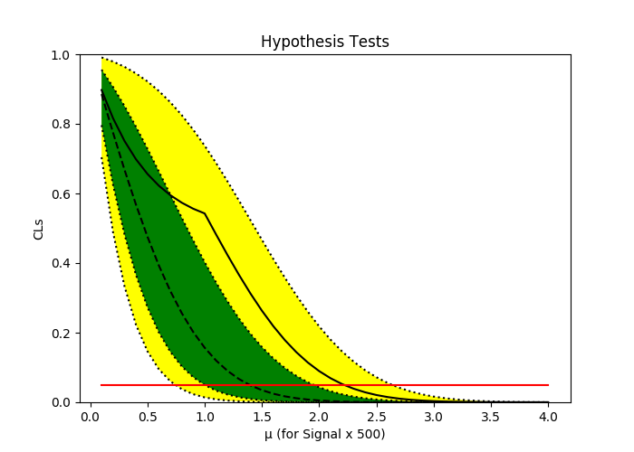
    # Visualize the "Brazil band"
    fig, ax = plt.subplots()
    fig.set_size_inches(7, 5)

    ax.set_title("Hypothesis Tests")
    ax.set_ylabel("CLs")
    ax.set_xlabel(f"µ (for Signal x {scale_factor})")

    pyhf.contrib.viz.brazil.plot_results(ax, poi_tests, hypo_tests)
    fig.savefig("brazil_band.pdf")


if __name__ == "__main__":
    main()

输出

信号需要缩放的值可以通过尝试几个缩放因子值来确定，直到mu=1的信号强度的CLs值开始看起来合理(比1e-3更大的值)。在这个特殊的例子中，500的比例因子似乎没问题。

非标度信号强度的上限就是观察到的极限除以尺度因子，在这种情况下没有明显的灵敏度。

(example) $ python answer.py 
Observed CLs for µ=1: 0.54
-----
Expected (-2 σ) CLs for µ=1: 0.014
Expected (-1 σ) CLs for µ=1: 0.049
Expected        CLs for µ=1: 0.157
Expected (1 σ) CLs for µ=1: 0.403
Expected (2 σ) CLs for µ=1: 0.737

Performing hypothesis tests

Observed Limit on µ: 2.22
-----
Expected (-2 σ) Limit on µ: 0.746
Expected (-1 σ) Limit on µ: 0.998
Expected        Limit on µ: 1.392
Expected (1 σ) Limit on µ: 1.953
Expected (2 σ) Limit on µ: 2.638

​

​