用两个线性函数和Python中的一个断点进行分段拟合

Question

我想用两个线性函数(破幂律)来拟合我的数据，其中一个是用户给定的断点。目前，我正在使用来自curve_fit模块的scipy.optimize函数。这是我的数据集频率，联合数据，错误

这是我的代码：

import numpy as np
from scipy.optimize import curve_fit
import matplotlib.pyplot as plt


freqs=np.loadtxt('binf11.dat')
binys=np.loadtxt('binp11.dat')
errs=np.loadtxt('bine11.dat')


def brkPowLaw(xArray, breakp, slopeA, offsetA, slopeB):
    returnArray = []
    for x in xArray:
        if x <= breakp:
            returnArray.append(slopeA * x + offsetA)
        elif x>breakp:           
            returnArray.append(slopeB * x + offsetA)
    return returnArray

#define initial guesses, breakpoint=-3.2
a_fit,cov=curve_fit(brkPowLaw,freqs,binys,sigma=errs,p0=(-3.2,-2.0,-2.0,-2.0))


modelPredictions = brkPowLaw(freqs, *a_fit) 


plt.errorbar(freqs, binys, yerr=errs, fmt='kp',fillstyle='none',elinewidth=1)
plt.xlim(-5,-2)
plt.plot(freqs,modelPredictions,'r')

第二线性函数的偏移量被设置为等于第一线性函数的偏移量。

它看起来很管用，但我觉得它很合适：

​

​

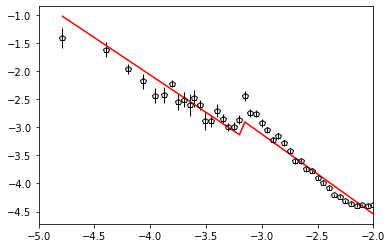
现在，我认为brkPowLaw函数中的条件应该足够了，但事实并非如此。我想要的是，用第一个线性方程把数据拟合到一个选定的临界点，然后从这个临界点再进行第二个线性拟合，但是没有驼峰，就像它在图中显示的那样，因为现在它看起来有两个断点，而不是一个和三个线性函数来拟合，这不是我所期望的，也不是我想要的。

我想要的是，当第一个线性拟合结束时，第二个线性拟合从第一个线性拟合结束的点开始。

我尝试过使用numpy.piecewise函数，但没有得到合理的结果，我研究了一些主题( 像这样或这 )，但是我没有设法使我的脚本工作。

谢谢您抽时间见我

Answer 1

这将是我的方法，不是线性而是二次函数。

import matplotlib.pyplot as plt
import numpy as np
from scipy.optimize import curve_fit

def soft_step(x, s): ### not my usual np.tanh() ...OMG
    return 1+ 0.5 * s * x / np.sqrt( 1 + ( s * x )**2 )

### for the looks of the data I decided to go for two parabolas with 
### one discontinuity
def fit_func( x, a0, b0, c0, a1, b1, c1, x0, s ):
    out  = ( a0 * x**2 + b0 * x + c0 ) * ( 1 - soft_step( x - x0, s ) )
    out += ( a1 * x**2 + b1 * x + c1 ) * soft_step( x - x0, s )
    return out

### with global parameter for iterative fit
### if using least_squares one could avoid globals
def fit_short( x, a0, b0, c0, a1, b1, c1, x0 ):
    global stepwidth
    return fit_func( x, a0, b0, c0, a1, b1, c1, x0, stepwidth )

### getting data
xl = np.loadtxt( "binf11.dat" )
yl = np.loadtxt( "binp11.dat" )
el = np.loadtxt( "bine11.dat" )

### check for initial values
p0 = [ 0, -2,-11, 0, -2, -9, -3, 10 ]
xth = np.linspace( -5.5, -1.5, 250 )
yth = np.fromiter( ( fit_func(x, *p0 ) for x in xth ), np.float )

### initial fit
sol, pcov = curve_fit( fit_func, xl, yl, sigma=el, p0=p0, absolute_sigma=True )
yft = np.fromiter( ( fit_func( x, *sol ) for x in xth ), np.float )
sol=sol[: -1]

###iterating with fixed and decreasing softness in the step
for stepwidth in range(10,55,5):
    sol, pcov = curve_fit( fit_short, xl, yl, sigma=el, p0=sol, absolute_sigma=True )
    ### printing the step position
    print sol[-1]
yiter = np.fromiter( ( fit_short(x, *sol ) for x in xth ), np.float )
print sol

###plotting
fig = plt.figure()
ax = fig.add_subplot( 1, 1, 1 )
# ~ax.plot( xth, yth ) ### no need to show start parameters
ax.plot( xth, yft ) ### first fit with variable softness
ax.plot( xth, yiter ) ### last fit with fixed softness of 50
ax.errorbar( xl, yl, el, marker='o', ls='' ) ### data
plt.show()

这意味着：

-3.1762721614559712
-3.1804393481217477
-3.1822672190583603
-3.183493292415725
-3.1846976088390333
-3.185974760198917
-3.1872472903175266
-3.188427041827035
-3.1894705102541843
[ -0.78797351  -5.33255174 -12.48258537   0.53024954   1.14252783 -4.44589397  -3.18947051]

和

​

​

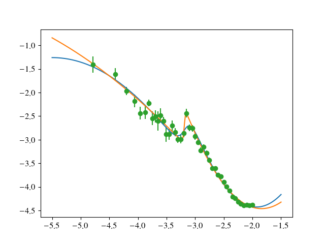
把跳跃速度定在-3.189