文章/答案/技术大牛

发布

社区首页 >问答首页 >将时间序列数据聚合成散点图

问将时间序列数据聚合成散点图
EN

Stack Overflow用户

提问于 2020-08-04 03:14:12

回答 2查看 1.6K关注 0票数 3

我想为我的时间序列数据绘制时间序列散点图，其中我的数据有分类列，需要先按组进行聚合才能生成绘图数据，然后使用seaborn或matplotlib绘制散点图。我的数据是产品销售价格的时间序列数据，我希望看到每个产品所有者的价格趋势在不同的市场门槛沿时间。我尝试使用pandas.pivot_table，groupby来生成绘图数据，但没有得到我想要的绘图。

可复制数据

这是我使用的示例产品数据；在哪里，我希望看到每个经销商关于threshold的不同蛋白质类型的价格趋势。

我的尝试

下面是我目前为绘制绘图数据而聚合数据的尝试，但它并没有给出正确的绘图。我打赌我收集绘图数据的方法是不正确的。有人能告诉我怎样才能得到想要的情节吗？

import pandas as pd
import numpy as np
import matplotlib.pyplot as plt
import seaborn as sn

mydf = pd.read_csv('foo.csv')
mydf=mydf.drop(mydf.columns[0], axis=1)
mydf['expected_price'] = mydf['price']*76/mydf['threshold']

g = mydf.groupby(['dealer','protein_type'])
newdf= g.apply(lambda x: pd.Series([np.average(x['threshold'])])).unstack()

但是上面的尝试不起作用，因为我想要绘制每个经销商在不同的protein_type上的市场购买价格的数据，以及每天的时间序列中不同的threshold。我不知道处理这个时间序列的最好方法是什么。有人能给我建议或者纠正我怎么做才对吗？

我也尝试过pandas/pivot_table来聚合我的数据，但它仍然不代表绘图数据。

pv_df= pd.pivot_table(mydf, index=['date'], columns=['dealer', 'protein_type', 'threshold'],values=['price'])
pv_df= pv_df.fillna(0)
pv_df.groupby(['dealer', 'protein_type', 'threshold'])['price'].unstack().reset_index()

但上述尝试仍未奏效。另外，在我的数据中，日期是不连续的，所以我假设我可以绘制每月时间序列线图。

我制作情节的尝试

以下是我制作剧情的尝试：

def scatterplot(x_data, y_data, x_label, y_label, title):
    fig, ax = plt.subplots()
    ax.scatter(x_data, y_data, s = 30, color = '#539caf', alpha = 0.75)

    ax.set_title(title)
    ax.set_xlabel(x_label)
    ax.set_ylabel(y_label)
    fig.autofmt_xdate()

期望输出

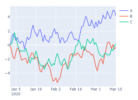
我想要线图或散点图，其中x轴显示每月时间序列，而y轴显示每个不同的protein_type在不同的threshold值上的价格，每个不同的经销商沿着月时间序列。下面是我想要的可能的线条图：

matplotlib

time-series

seaborn

python

pandas

回答 2

Stack Overflow用户

回答已采纳

发布于 2020-08-04 09:13:28

用threshold更新

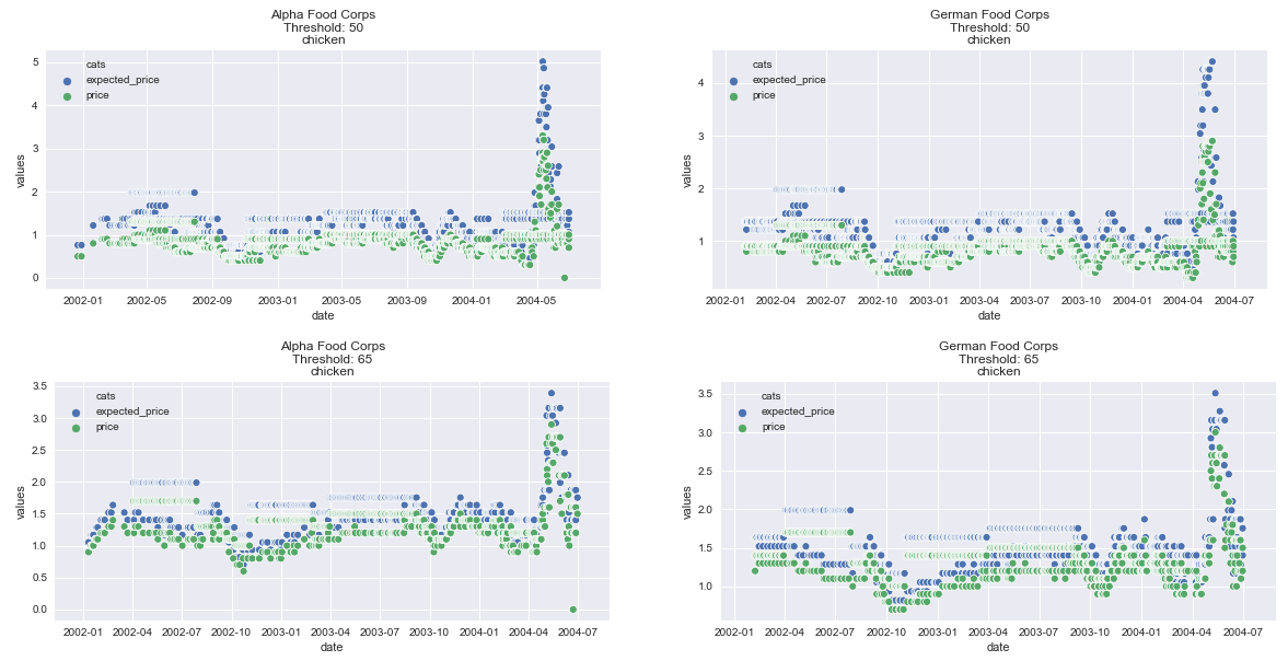
备选案文1

此选项是在看到选项1的结果后实现的。
- 在这些情节中有许多无法解释的信息，而且它们没有清楚地提供数据。
为了清楚地显示数据，每个地块应该只包含一个dealer、一个threshold和一个protein_type的三个维度的数据(例如，dealer、values和cats)。

import pandas as pd
import matplotlib.pyplot as plt
import seaborn as sns
from datetime import timedelta

# read the data in and parse the date column and set threshold as a str
df = pd.read_csv('data/so_data/2020-08-03 63239708/mydf.csv', parse_dates=['date'])

# calculate expected price
df['expected_price'] = df.price*76/df.threshold

# set threshold as a category
df.threshold = df.threshold.astype('category')

# set the index
df = df.set_index(['date', 'dealer', 'protein_type', 'threshold'])

# form the dataframe into a long form
dfl = df.drop(columns=['destination', 'quantity']).stack().reset_index().rename(columns={'level_4': 'cats', 0: 'values'})

# plot
for pt in dfl.protein_type.unique():
    for t in dfl.threshold.unique():
        data = dfl[(dfl.protein_type == pt) & (dfl.threshold == t)]
        if not data.empty:
            utc = len(data.threshold.unique())
            f, axes = plt.subplots(nrows=utc, ncols= 2, figsize=(20, 4), squeeze=False)
            for j in range(utc):
                for i, d in enumerate(dfl.dealer.unique()):
                    data_d = data[data.dealer == d].sort_values(['cats', 'date']).reset_index(drop=True)
                    p = sns.scatterplot('date', 'values', data=data_d, hue='cats', ax=axes[j, i])
                    if not data_d.empty:
                        p.set_title(f'{d}\nThreshold: {t}\n{pt}')
                        p.set_xlim(data_d.date.min() - timedelta(days=60), data_d.date.max() + timedelta(days=60))
                    else:
                        p.set_title(f'{d}: No Data Available\nThreshold: {t}\n{pt}')
                    
            plt.show()

前四样地

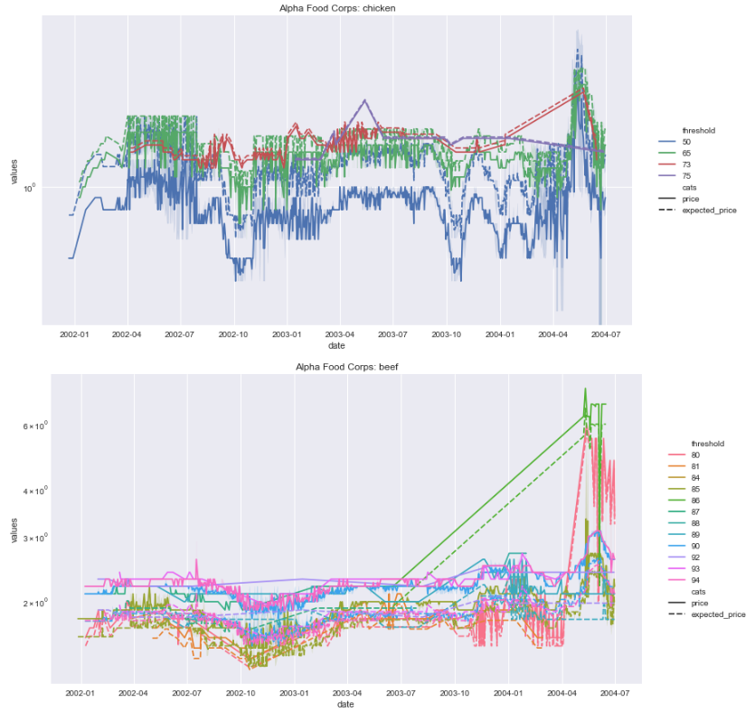
选项2

这导致了4个不同的图形，threshold作为一个category类型。
必须首先将threshold保留为expected_price计算的int，然后进行转换。
请注意，我的数据没有额外的未命名列，因此仍然需要删除该列，这在下面的代码中没有显示。

import pandas as pd
import matplotlib.pyplot as plt
import seaborn as sns

# read the data in and parse the date column and set threshold as a str
df = pd.read_csv('data/so_data/2020-08-03 63239708/mydf.csv', parse_dates=['date'])

# calculate expected price
df['expected_price'] = df.price*76/df.threshold

# set threshold as a category
df.threshold = df.threshold.astype('category')

# set the index
df = df.set_index(['date', 'dealer', 'protein_type', 'threshold'])

# form the dataframe into a long form
dfl = df.drop(columns=['destination', 'quantity']).stack().reset_index().rename(columns={'level_4': 'cats', 0: 'values'})

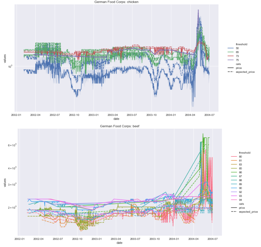
# plot four plots with threshold
for d in dfl.dealer.unique():
    for pt in dfl.protein_type.unique():
        plt.figure(figsize=(13, 7))
        data = dfl[(dfl.protein_type == pt) & (dfl.dealer == d)]
        sns.lineplot('date', 'values', data=data, hue='threshold', style='cats')
        plt.yscale('log')
        plt.title(f'{d}: {pt}')
        plt.legend(bbox_to_anchor=(1.04,0.5), loc="center left", borderaxespad=0)

原始的没有threshold作为一个类别

我不明白你在做什么：
- newdf= g.apply(lambda x: pd.Series([np.average(x['threshold'])])).unstack()
- 我不认为这与主要问题是不可分割的，那就是绘制数据
首先，需要将数据格式转换为长格式，并删除'destination'。
在一个单一的图形上有很多维度要绘制
- x='date'，y='values'，hue='cats'，style='dealer'
- 'protein_type'需要一个单独的数字
- 但是，包括'dealer'在内的数据重叠程度很高，因此需要4幅图。

DataFrame设置：

请注意，我的数据没有额外的未命名列，因此仍然需要删除该列，这在下面的代码中没有显示。
使用pandas.DataFrame.stack将数据转换为长表单

备选案文1：

import pandas as pd
import matplotlib.pyplot as plt
import seaborn as sns

# read the data in
df = pd.read_csv('data/so_data/2020-08-03 63239708/mydf.csv', parse_dates=['date'])

# your calculation
df['expected_price'] = df['price']*76/df['threshold']

# set the index
df = df.set_index(['date', 'dealer', 'protein_type'])

# form the dataframe into a long form
dfl = df.drop(columns=['destination']).stack().reset_index().rename(columns={'level_3': 'cats', 0: 'values'})

# display(dfl.head())
        date            dealer protein_type            cats    values
0 2001-12-22  Alpha Food Corps      chicken       threshold     50.00
1 2001-12-22  Alpha Food Corps      chicken        quantity  39037.00
2 2001-12-22  Alpha Food Corps      chicken           price      0.50
3 2001-12-22  Alpha Food Corps      chicken  expected_price      0.76
4 2001-12-27  Alpha Food Corps         beef       threshold     85.00

备选方案2:滚动平均数

pandas.DataFrame.groupby和pandas.DataFrame.rolling mean，然后是.stack。

df = pd.read_csv('data/so_data/2020-08-03 63239708/mydf.csv', parse_dates=['date'])
df['expected_price'] = df['price']*76/df['threshold']
df = df.set_index('date')

# groupby aggregate rolling mean and stack
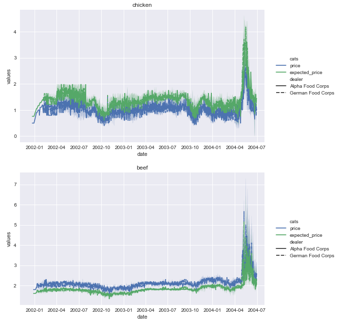
dfl = df.groupby(['dealer', 'protein_type'])[['expected_price', 'price']].rolling(7).mean().stack().reset_index().rename(columns={'level_3': 'cats', 0: 'values'})

备选案文1:两个地块

'dealer'数据是相似的差异化(价格串通吗？)

for pt in dfl.protein_type.unique():
    plt.figure(figsize=(9, 5))
    data = dfl[dfl.protein_type == pt]
    sns.lineplot('date', 'values', data=data, hue='cats', style='dealer')
    plt.xlim(datetime(2001, 11, 1), datetime(2004, 8, 1))
    plt.yscale('log')
    plt.title(pt)
    plt.legend(bbox_to_anchor=(1.04,0.5), loc="center left", borderaxespad=0)

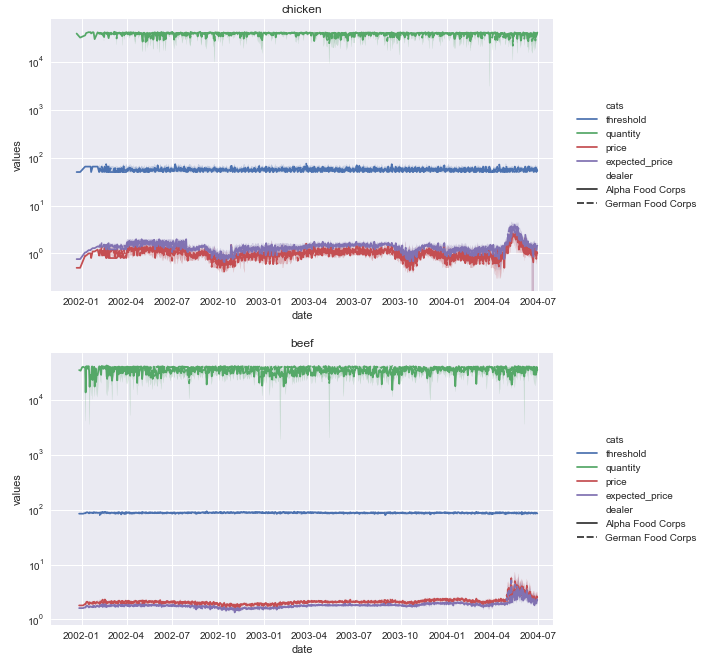
即使只有'price'和'expected_price'，也无法确定'dealer'。

备选案文2:四个地块

seaborn.FacetGrid

g = sns.FacetGrid(data=dfl, col='dealer', row='protein_type', hue='cats', height=5, aspect=1.5)
g.map(sns.lineplot, 'date', 'values').add_legend()
plt.yscale('log')
g.set_xticklabels(rotation=90)

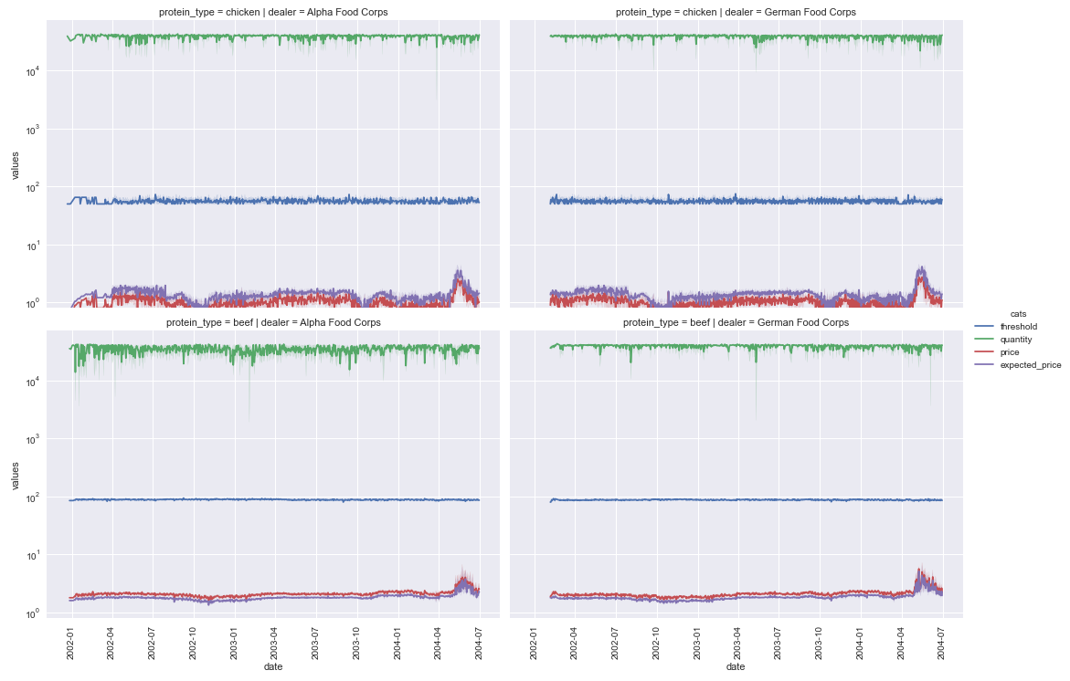
滚动平均值数据图

嵌套环

这将产生一列4位数，首先为dealer选择，然后为protein_type选择。
可选地，交换dealer和protein的顺序

for d in dfl.dealer.unique():
    for pt in dfl.protein_type.unique():
        plt.figure(figsize=(10, 5))
        data = dfl[(dfl.protein_type == pt) & (dfl.dealer == d)]
        sns.lineplot('date', 'values', data=data, hue='cats')
        plt.xlim(datetime(2001, 11, 1), datetime(2004, 8, 1))
        plt.yscale('log')
        plt.title(f'{d}: {pt}')
        plt.legend(bbox_to_anchor=(1.04,0.5), loc="center left", borderaxespad=0)

CSV样本：

date,dealer,threshold,quantity,price,protein_type,destination
2001-12-22,Alpha Food Corps,50,39037,0.5,chicken,UK
2001-12-27,Alpha Food Corps,85,35432,1.8,beef,UK
2001-12-29,Alpha Food Corps,50,32142,0.5,chicken,UK
2001-12-30,Alpha Food Corps,85,34516,1.8,beef,UK
2002-01-02,Alpha Food Corps,85,39930,1.8,beef,UK
2002-01-04,Alpha Food Corps,85,40709,1.8,beef,UK
2002-01-08,Alpha Food Corps,94,37641,2.2,beef,UK
2002-01-08,Alpha Food Corps,85,37545,1.8,beef,UK
2002-01-08,Alpha Food Corps,85,37564,1.8,beef,UK
2002-01-08,Alpha Food Corps,85,37607,1.8,beef,UK
2002-01-08,Alpha Food Corps,85,41706,1.8,beef,UK
2002-01-08,Alpha Food Corps,90,41628,2.1,beef,UK
2002-01-08,Alpha Food Corps,65,35720,0.9,chicken,UK
2002-01-09,Alpha Food Corps,94,1581,2.2,beef,UK
2002-01-09,Alpha Food Corps,85,11426,1.8,beef,UK
2002-01-09,Alpha Food Corps,85,37489,1.8,beef,UK
2002-01-09,Alpha Food Corps,90,15630,2.1,beef,UK
2002-01-09,Alpha Food Corps,80,3136,1.6,beef,UK
2002-01-10,Alpha Food Corps,85,41919,1.8,beef,UK
2002-01-10,Alpha Food Corps,90,39932,2.1,beef,UK
2002-01-10,Alpha Food Corps,90,41665,2.1,beef,UK
2002-01-10,Alpha Food Corps,90,41860,2.1,beef,UK
2002-01-10,Alpha Food Corps,65,39879,0.9,chicken,UK
2002-01-10,Alpha Food Corps,65,39884,0.9,chicken,UK
2002-01-11,Alpha Food Corps,90,37613,2.1,beef,UK
2002-01-12,Alpha Food Corps,90,41855,2.1,beef,UK
2002-01-13,Alpha Food Corps,90,37585,2.1,beef,UK
2002-01-15,Alpha Food Corps,85,41618,1.8,beef,UK
2002-01-15,Alpha Food Corps,85,41721,1.8,beef,UK
2002-01-15,Alpha Food Corps,85,41869,1.8,beef,UK
2002-01-15,Alpha Food Corps,85,41990,1.8,beef,UK
2002-01-15,Alpha Food Corps,90,41744,2.1,beef,UK
2002-01-15,Alpha Food Corps,90,41936,2.1,beef,UK
2002-01-15,Alpha Food Corps,65,41684,1.0,chicken,UK
2002-01-15,Alpha Food Corps,65,41776,1.0,chicken,UK
2002-01-16,Alpha Food Corps,94,35891,2.2,beef,UK
2002-01-16,Alpha Food Corps,85,39985,1.8,beef,UK
2002-01-16,Alpha Food Corps,85,41754,1.8,beef,UK
2002-01-16,Alpha Food Corps,85,41811,1.8,beef,UK
2002-01-16,Alpha Food Corps,90,39838,2.1,beef,UK
2002-01-16,Alpha Food Corps,80,3244,1.7,beef,UK
2002-01-17,Alpha Food Corps,94,22245,2.2,beef,UK
2002-01-17,Alpha Food Corps,85,5186,1.8,beef,UK
2002-01-17,Alpha Food Corps,90,2016,2.1,beef,UK
2002-01-17,Alpha Food Corps,90,40875,2.1,beef,UK
2002-01-17,Alpha Food Corps,65,41440,1.0,chicken,UK
2002-01-18,Alpha Food Corps,94,12525,2.2,beef,UK
2002-01-18,Alpha Food Corps,94,31325,2.2,beef,UK
2002-01-18,Alpha Food Corps,85,15486,1.8,beef,UK
2002-01-18,Alpha Food Corps,85,29992,1.8,beef,UK
2002-01-18,Alpha Food Corps,85,39938,1.8,beef,UK
2002-01-18,Alpha Food Corps,85,41777,1.8,beef,UK
2002-01-18,Alpha Food Corps,90,9475,2.1,beef,UK
2002-01-18,Alpha Food Corps,90,9960,2.1,beef,UK
2002-01-18,Alpha Food Corps,90,41676,2.1,beef,UK
2002-01-18,Alpha Food Corps,90,41816,2.1,beef,UK
2002-01-18,Alpha Food Corps,90,42036,2.1,beef,UK
2002-01-18,Alpha Food Corps,65,41673,1.0,chicken,UK
2002-01-19,Alpha Food Corps,85,19961,1.8,beef,UK
2002-01-19,Alpha Food Corps,90,19955,2.1,beef,UK
2002-01-19,Alpha Food Corps,90,40437,2.1,beef,UK
2002-01-19,Alpha Food Corps,65,41574,1.0,chicken,UK
2002-01-19,Alpha Food Corps,65,41700,1.0,chicken,UK
2002-01-20,Alpha Food Corps,94,23278,2.2,beef,UK
2002-01-20,Alpha Food Corps,85,9230,1.8,beef,UK
2002-01-20,Alpha Food Corps,85,38842,1.8,beef,UK
2002-01-20,Alpha Food Corps,90,9173,2.1,beef,UK
2002-01-20,Alpha Food Corps,90,38608,2.1,beef,UK
2002-01-20,Alpha Food Corps,50,39191,0.8,chicken,UK
2002-01-22,Alpha Food Corps,94,41741,2.2,beef,UK
2002-01-22,Alpha Food Corps,85,39879,1.8,beef,UK
2002-01-22,Alpha Food Corps,85,41683,1.8,beef,UK
2002-01-22,Alpha Food Corps,85,41958,1.8,beef,UK
2002-01-22,Alpha Food Corps,90,41833,2.1,beef,UK
2002-01-23,Alpha Food Corps,94,20294,2.2,beef,UK
2002-01-23,Alpha Food Corps,85,15553,1.8,beef,UK
2002-01-23,Alpha Food Corps,85,40753,1.8,beef,UK
2002-01-23,Alpha Food Corps,85,41740,1.8,beef,UK
2002-01-23,Alpha Food Corps,90,1892,2.1,beef,UK
2002-01-23,Alpha Food Corps,90,39850,2.1,beef,UK
2002-01-23,Alpha Food Corps,80,3231,1.7,beef,UK
2002-01-23,Alpha Food Corps,65,41415,1.1,chicken,UK
2002-01-24,Alpha Food Corps,90,35473,2.1,beef,UK
2002-01-24,Alpha Food Corps,90,41824,2.1,beef,UK
2002-01-24,Alpha Food Corps,65,41721,1.1,chicken,UK
2002-01-25,Alpha Food Corps,85,19983,1.8,beef,UK
2002-01-25,Alpha Food Corps,85,35823,1.8,beef,UK
2002-01-25,Alpha Food Corps,90,19949,2.1,beef,UK
2002-01-25,Alpha Food Corps,90,41800,2.1,beef,UK
2002-01-25,Alpha Food Corps,65,40990,1.1,chicken,UK
2002-01-26,Alpha Food Corps,90,39938,2.1,beef,UK
2002-01-26,Alpha Food Corps,90,40641,2.1,beef,UK
2002-01-26,Alpha Food Corps,90,41550,2.1,beef,UK
2002-01-27,Alpha Food Corps,94,16589,2.2,beef,UK
2002-01-27,Alpha Food Corps,85,11669,1.8,beef,UK
2002-01-27,Alpha Food Corps,90,24982,2.1,beef,UK
2002-01-27,Alpha Food Corps,65,29819,1.1,chicken,UK
2002-01-29,Alpha Food Corps,94,37516,2.2,beef,UK
2002-01-29,Alpha Food Corps,85,37378,1.8,beef,UK
2002-01-29,Alpha Food Corps,85,37535,1.8,beef,UK
2002-01-29,Alpha Food Corps,85,40174,1.8,beef,UK
2002-01-29,Alpha Food Corps,90,37831,2.1,beef,UK
2002-01-30,Alpha Food Corps,94,34435,2.2,beef,UK
2002-01-30,Alpha Food Corps,94,39640,2.2,beef,UK
2002-01-30,Alpha Food Corps,85,1619,1.8,beef,UK
2002-01-30,Alpha Food Corps,85,3058,1.8,beef,UK
2002-01-30,Alpha Food Corps,85,20929,1.8,beef,UK
2002-01-30,Alpha Food Corps,90,3641,2.1,beef,UK
2002-01-30,Alpha Food Corps,90,20974,2.1,beef,UK
2002-01-30,Alpha Food Corps,90,31160,2.1,beef,UK
2002-01-30,Alpha Food Corps,92,38189,2.3,beef,UK
2002-01-31,Alpha Food Corps,94,8804,2.2,beef,UK
2002-01-31,Alpha Food Corps,85,17398,1.8,beef,UK
2002-01-31,Alpha Food Corps,90,13963,2.1,beef,UK
2002-01-31,Alpha Food Corps,90,37673,2.1,beef,UK
2002-01-31,Alpha Food Corps,90,40330,2.1,beef,UK
2002-01-31,Alpha Food Corps,90,40511,2.2,beef,UK
2002-01-31,Alpha Food Corps,80,38290,1.9,beef,UK
2002-01-31,Alpha Food Corps,92,37193,2.3,beef,UK
2002-02-01,Alpha Food Corps,94,5011,2.2,beef,UK
2002-02-01,Alpha Food Corps,85,18783,1.8,beef,UK
2002-02-01,Alpha Food Corps,85,41827,1.8,beef,UK
2002-02-01,Alpha Food Corps,90,16394,2.1,beef,UK
2002-02-01,Alpha Food Corps,90,23013,2.1,beef,UK
2002-02-01,Alpha Food Corps,90,39923,2.1,beef,UK
2002-02-01,Alpha Food Corps,90,41417,2.1,beef,UK
2002-02-01,Alpha Food Corps,80,15592,1.7,beef,UK
2002-02-01,Alpha Food Corps,80,38364,1.9,beef,UK
2002-02-01,Alpha Food Corps,92,37605,2.3,beef,UK
2002-02-01,Alpha Food Corps,92,39234,2.3,beef,UK
2002-02-02,Alpha Food Corps,90,34578,2.1,beef,UK
2002-02-02,Alpha Food Corps,90,41661,2.1,beef,UK
2002-02-02,Alpha Food Corps,80,3157,1.7,beef,UK
2002-02-02,Alpha Food Corps,65,41272,1.2,chicken,UK
2002-02-02,Alpha Food Corps,65,41503,1.2,chicken,UK
2002-02-02,Alpha Food Corps,92,36207,2.3,beef,UK
2002-02-05,Alpha Food Corps,94,41559,2.2,beef,UK
2002-02-05,Alpha Food Corps,85,41549,1.8,beef,UK
2002-02-05,Alpha Food Corps,85,41753,1.8,beef,UK
2002-02-05,Alpha Food Corps,85,41908,1.8,beef,UK
2002-02-05,Alpha Food Corps,90,39813,2.1,beef,UK
2002-02-05,Alpha Food Corps,90,41526,2.1,beef,UK
2002-02-05,German Food Corps,80,36031,1.9,beef,UK
2002-02-05,German Food Corps,50,38538,0.9,chicken,UK
2002-02-05,Alpha Food Corps,50,38772,0.9,chicken,UK
2002-02-05,German Food Corps,50,39099,0.9,chicken,UK
2002-02-05,German Food Corps,50,39132,0.9,chicken,UK
2002-02-05,German Food Corps,50,39207,0.9,chicken,UK
2002-02-06,Alpha Food Corps,85,41947,1.8,beef,UK
2002-02-06,German Food Corps,80,37287,1.9,beef,UK
2002-02-06,Alpha Food Corps,89,43201,2.1,beef,UK
2002-02-06,German Food Corps,50,38553,0.9,chicken,UK
2002-02-06,German Food Corps,50,38837,0.9,chicken,UK
2002-02-06,Alpha Food Corps,50,38985,0.9,chicken,UK
2002-02-06,German Food Corps,65,40386,1.4,chicken,UK
2002-02-06,Alpha Food Corps,65,41851,1.2,chicken,UK
2002-02-06,Alpha Food Corps,92,38405,2.3,beef,UK
2002-02-06,German Food Corps,73,37731,1.5,chicken,UK
2002-02-07,Alpha Food Corps,85,41097,1.9,beef,UK
2002-02-07,Alpha Food Corps,90,39582,2.1,beef,UK
2002-02-07,German Food Corps,65,38832,1.4,chicken,UK
2002-02-07,German Food Corps,50,39269,0.9,chicken,UK
2002-02-07,German Food Corps,50,40129,0.9,chicken,UK
2002-02-07,German Food Corps,50,41124,0.8,chicken,UK
2002-02-07,German Food Corps,65,41739,1.2,chicken,UK
2002-02-08,Alpha Food Corps,85,20034,1.8,beef,UK
2002-02-08,German Food Corps,85,33503,1.9,beef,UK
2002-02-08,German Food Corps,85,40780,1.9,beef,UK
2002-02-08,Alpha Food Corps,90,19913,2.1,beef,UK
2002-02-08,Alpha Food Corps,90,36682,2.1,beef,UK
2002-02-08,Alpha Food Corps,90,41624,2.1,beef,UK
2002-02-08,German Food Corps,65,37503,1.4,chicken,UK
2002-02-08,German Food Corps,50,38973,0.9,chicken,UK
2002-02-08,German Food Corps,50,39069,0.9,chicken,UK
2002-02-08,German Food Corps,50,40697,0.9,chicken,UK
2002-02-08,German Food Corps,92,36103,2.3,beef,UK
2002-02-08,Alpha Food Corps,92,38278,2.3,beef,UK
2002-02-09,Alpha Food Corps,90,39842,2.1,beef,UK
2002-02-09,Alpha Food Corps,90,16553,2.3,beef,UK
2002-02-09,Alpha Food Corps,80,18739,1.9,beef,UK
2002-02-09,German Food Corps,80,36349,1.9,beef,UK
2002-02-09,German Food Corps,65,35238,1.4,chicken,UK
2002-02-09,German Food Corps,50,38391,0.9,chicken,UK
2002-02-09,Alpha Food Corps,50,38819,0.9,chicken,UK
2002-02-09,German Food Corps,50,41691,0.9,chicken,UK
2002-02-09,Alpha Food Corps,92,40245,2.3,beef,UK
2002-02-09,German Food Corps,73,37323,1.5,chicken,UK
2002-02-09,German Food Corps,90,40312,2.2,beef,UK
2002-02-10,Alpha Food Corps,90,42108,2.1,beef,UK
2002-02-10,German Food Corps,65,37831,1.4,chicken,UK
2002-02-11,Alpha Food Corps,50,38591,0.9,chicken,UK
2002-02-12,Alpha Food Corps,94,41559,2.3,beef,UK
2002-02-12,Alpha Food Corps,85,40968,1.8,beef,UK
2002-02-12,Alpha Food Corps,85,41985,1.8,beef,UK
2002-02-12,German Food Corps,50,38931,0.9,chicken,UK
2002-02-12,German Food Corps,50,38986,0.9,chicken,UK
2002-02-12,German Food Corps,92,39684,2.3,beef,UK
2002-02-12,German Food Corps,73,36619,1.5,chicken,UK
2002-02-13,Alpha Food Corps,85,41291,1.8,beef,UK
2002-02-13,Alpha Food Corps,85,41892,1.8,beef,UK

票数 7

Stack Overflow用户

发布于 2020-08-04 09:20:31

在行图中，据我所知，您只能表示4个维度：

x轴，您可以将它用于date
y轴，您可以将其用于price
行色调，您可以将其用于threshold
行样式，您可以将其用于dealer

但是你要考虑到第五个维度：protein_type.为此，我建议使用一个子图，如下代码所示：

# import packages
import pandas as pd
import matplotlib.pyplot as plt
import seaborn as sns

# read dataframe
mydf = pd.read_csv('foo.csv')
mydf = mydf.drop(mydf.columns[0], axis = 1)

# convert 'date' type to datetime and sort values by threshold, then by date
mydf['date'] = pd.to_datetime(mydf['date'], format = '%m/%d/%Y')
mydf['threshold'] = mydf['threshold'].astype('category')
mydf.sort_values(['threshold', 'date'], inplace = True)

# set up subplots layout, one row for each threshold
fig, ax = plt.subplots(nrows = len(mydf['protein_type'].unique()),
                       ncols = 1,
                       figsize = (10, 10),
                       sharex = True)

# loop over protein_type
for i, protein_type in enumerate(mydf['protein_type'].unique(), 0):

    # filter dataframe
    df_filtered = mydf[mydf['protein_type'] == protein_type]

    # set up plot
    sns.lineplot(ax = ax[i],
                 data = df_filtered,
                 x = 'date',
                 y = 'price',
                 hue = 'threshold',
                 style = 'dealer',
                 legend = 'full',
                 ci = False)

    # set up subplot title and legend
    ax[i].set_title(f'Protein type = {protein_type}')
    ax[i].legend(bbox_to_anchor = (1.02, 1), loc = 'upper left')

# adjust general layout
plt.subplots_adjust(top = 0.95,
                    right = 0.85,
                    bottom = 0.05,
                    left = 0.05,
                    hspace = 0.15)

# show the plot
plt.show()

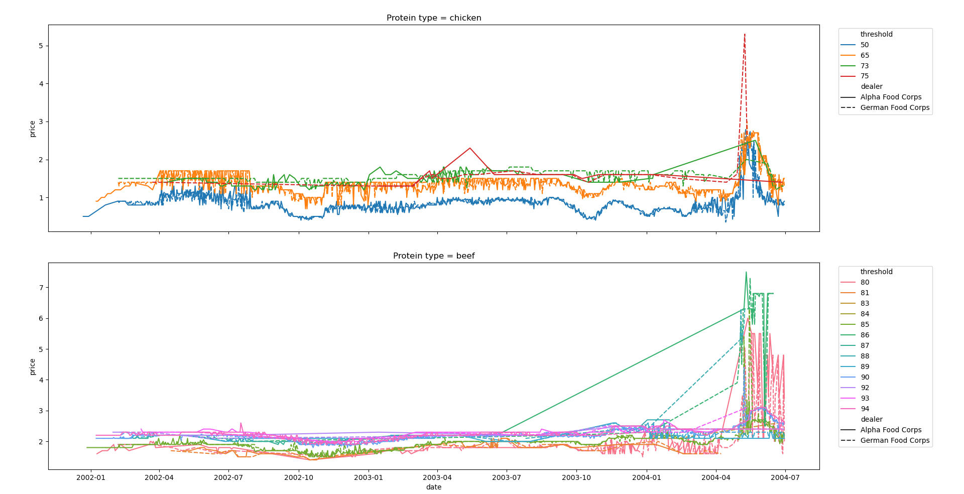
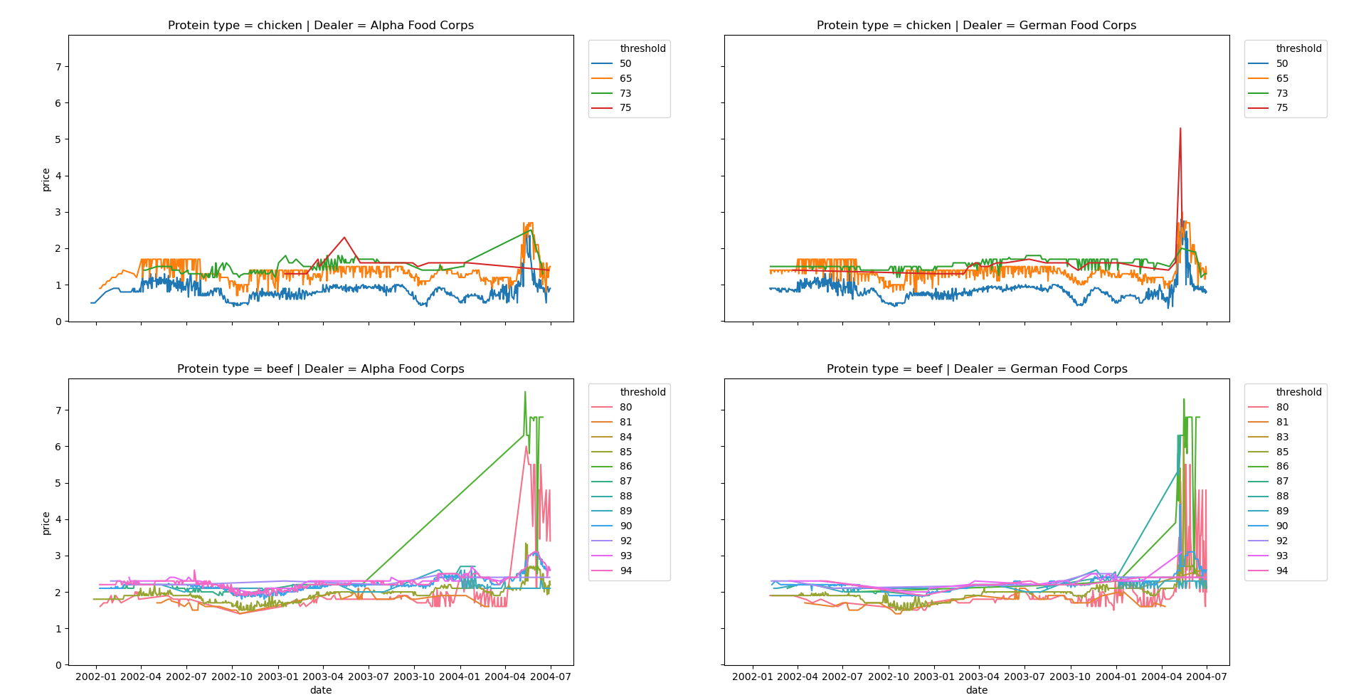
在上面的图中，很难理解经销商之间的差异，因此您可以在另一个子图网格中将它们分开，如下所示：

# import packages
import pandas as pd
import matplotlib.pyplot as plt
import seaborn as sns

# read dataframe
mydf = pd.read_csv('foo.csv')
mydf = mydf.drop(mydf.columns[0], axis = 1)

# convert 'date' type to datetime and sort values by threshold, then by date
mydf['date'] = pd.to_datetime(mydf['date'], format = '%m/%d/%Y')
mydf['threshold'] = mydf['threshold'].astype('category')
mydf.sort_values(['threshold', 'date'], inplace = True)

# set up subplots layout, one row for each threshold, one column for each dealer
fig, ax = plt.subplots(nrows = len(mydf['protein_type'].unique()),
                       ncols = len(mydf['dealer'].unique()),
                       figsize = (10, 10),
                       sharex = True,
                       sharey = True)

# loop over protein_type
for i, protein_type in enumerate(mydf['protein_type'].unique(), 0):

    # loop over dealer
    for j, dealer in enumerate(mydf['dealer'].unique(), 0):

        # filter dataframe
        df_filtered = mydf[(mydf['protein_type'] == protein_type) & (mydf['dealer'] == dealer)]

        # set up plot
        sns.lineplot(ax = ax[i, j],
                     data = df_filtered,
                     x = 'date',
                     y = 'price',
                     hue = 'threshold',
                     legend = 'full',
                     ci = False)

        # set up subplot title and legend
        ax[i, j].set_title(f'Protein type = {protein_type} | Dealer = {dealer}')
        ax[i, j].legend(bbox_to_anchor = (1.02, 1), loc = 'upper left')

# adjust general layout
plt.subplots_adjust(top = 0.95,
                    right = 0.9,
                    bottom = 0.05,
                    left = 0.05,
                    wspace = 0.3,
                    hspace = 0.2)

# show the plot
plt.show()

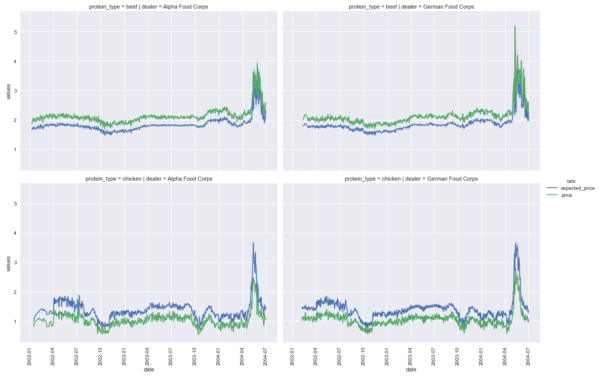
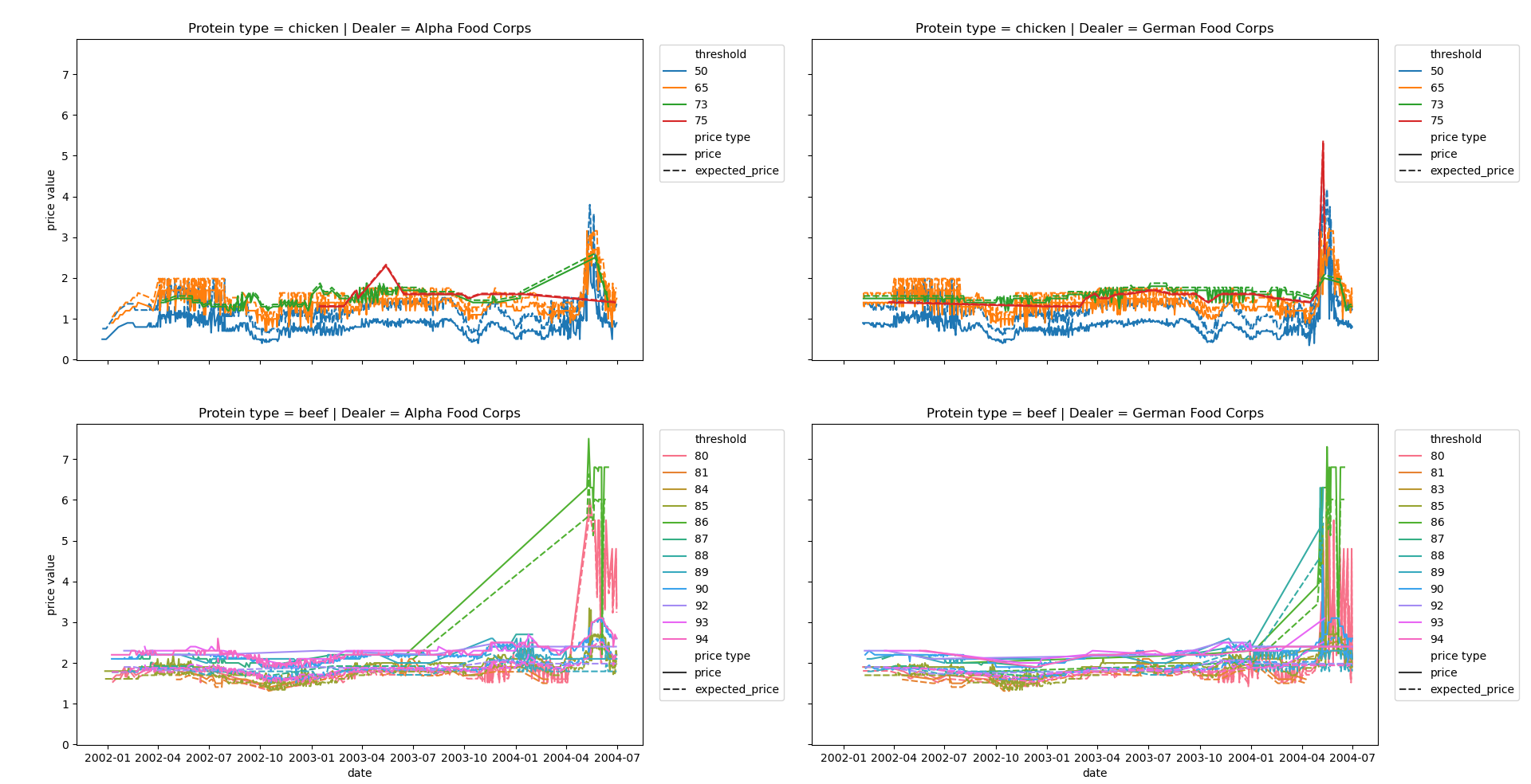
最后，如果要将price与expected_price进行比较，可以使用style维度来执行此任务。

这需要对dataframe进行不同的扩展:您必须将price和expected_price列堆叠在一个唯一的列中。您可以使用pd.melt方法来完成这一任务。

请检查下面的代码，作为参考：

# import packages
import pandas as pd
import matplotlib.pyplot as plt
import seaborn as sns

# read dataframe
mydf = pd.read_csv('foo.csv')
mydf = mydf.drop(mydf.columns[0], axis = 1)
mydf['expected_price'] = mydf['price']*76/mydf['threshold']

# convert 'date' type to datetime
mydf['date'] = pd.to_datetime(mydf['date'], format = '%m/%d/%Y')
mydf['threshold'] = mydf['threshold'].astype('category')

# reshape dataframe
mydf = pd.melt(frame = mydf,
               id_vars = ['date', 'dealer', 'threshold', 'quantity', 'protein_type', 'destination'],
               value_vars = ['price', 'expected_price'],
               var_name = 'price type',
               value_name = 'price value')

# sort values by threshold, then by date
mydf.sort_values(['threshold', 'date'], inplace = True)

# set up subplots layout, one row for each threshold, one column for each dealer
fig, ax = plt.subplots(nrows = len(mydf['protein_type'].unique()),
                       ncols = len(mydf['dealer'].unique()),
                       figsize = (10, 10),
                       sharex = True,
                       sharey = True)

# loop over protein_type
for i, protein_type in enumerate(mydf['protein_type'].unique(), 0):

    # loop over dealer
    for j, dealer in enumerate(mydf['dealer'].unique(), 0):

        # filter dataframe
        df_filtered = mydf[(mydf['protein_type'] == protein_type) & (mydf['dealer'] == dealer)]

        # set up plot
        sns.lineplot(ax = ax[i, j],
                     data = df_filtered,
                     x = 'date',
                     y = 'price value',
                     hue = 'threshold',
                     style = 'price type',
                     legend = 'full',
                     ci = False)

        # set up subplot title and legend
        ax[i, j].set_title(f'Protein type = {protein_type} | Dealer = {dealer}')
        ax[i, j].legend(bbox_to_anchor = (1.02, 1), loc = 'upper left')

# adjust general layout
plt.subplots_adjust(top = 0.95,
                    right = 0.9,
                    bottom = 0.05,
                    left = 0.05,
                    wspace = 0.3,
                    hspace = 0.2)

# show the plot
plt.show()

票数 3

页面原文内容由Stack Overflow提供。腾讯云小微IT领域专用引擎提供翻译支持

原文链接：

https://stackoverflow.com/questions/63239708

复制

相似问题

问将时间序列数据聚合成散点图
EN

回答 2

Stack Overflow用户

Stack Overflow用户

社区

活动

圈层

关于

腾讯云开发者

热门产品

热门推荐

更多推荐

问将时间序列数据聚合成散点图EN

回答 2

Stack Overflow用户

Stack Overflow用户

社区

活动

圈层

关于

腾讯云开发者

热门产品

热门推荐

更多推荐

问将时间序列数据聚合成散点图
EN