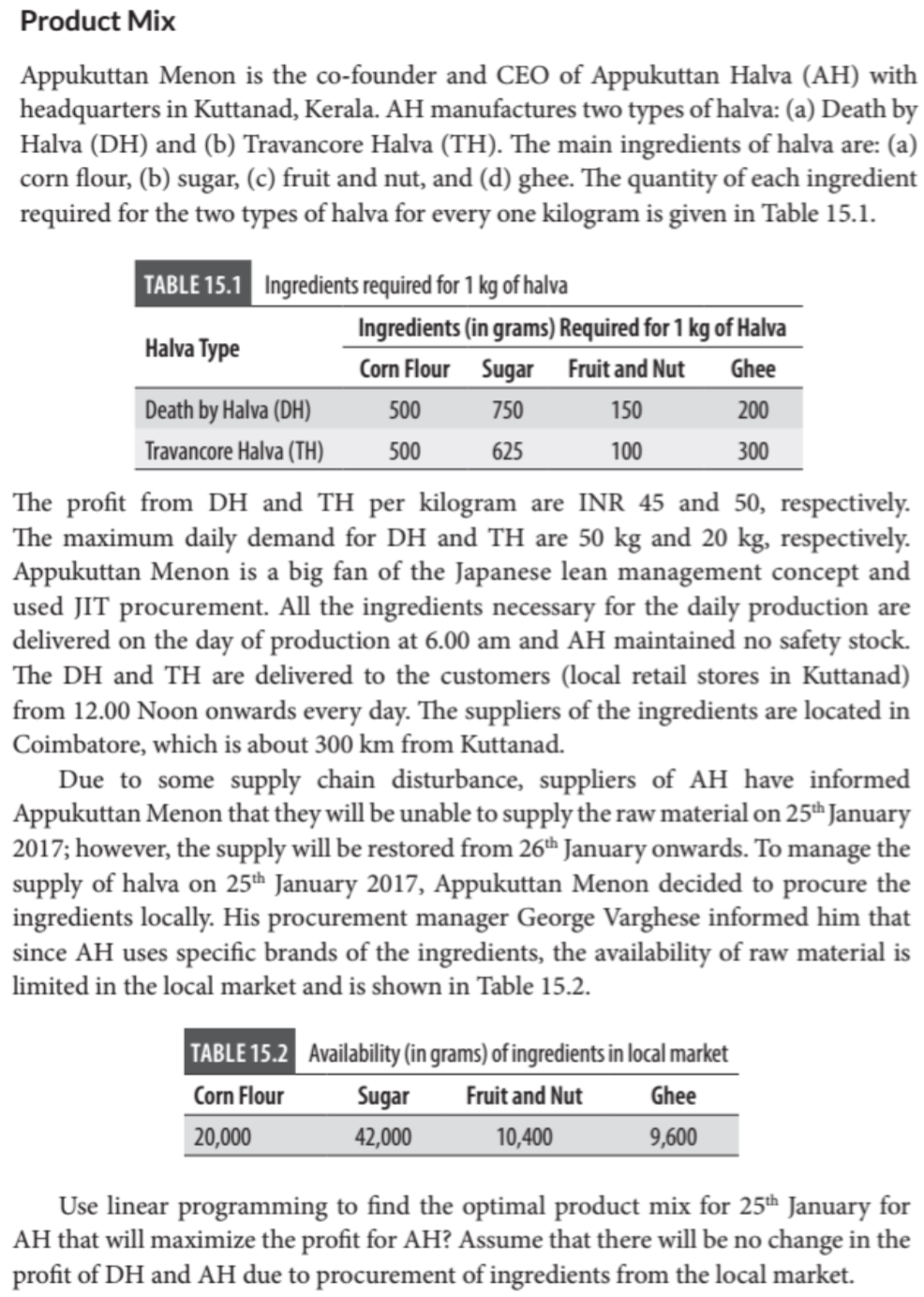
使用Gekko发布敏感性报告

Question

我用Gekko来解决一个简单的线性规划问题。我得到了一个最优解。当我试图获得敏感性报告时，我将面临以下错误。

@error: Degrees of Freedom Non-Zero for Sensitivity Analysis

然而，当我在excel中尝试同样的方法时，我没有看到任何问题。请帮我找出问题的确切原因。

问题陈述：

​

​

from gekko import GEKKO
model = GEKKO(remote=False)
model.options.SENSITIVITY = 1   # sensitivity analysis
model.options.SOLVER = 1        # change solver (1=APOPT, 3=IPOPT)
#Maximum demand and implicit contraints as upper bound and lower bound
x1 = model.Var(lb=0, ub=50) # Product DH
x2 = model.Var(lb=0, ub=20) # Product TH
#Objective function
model.Maximize(45*x1+50*x2) # Profit function
#Constraints
model.Equation(500*x1+500*x2<=20000) #Cornflour
model.Equation(750*x1+625*x2<=42000) #Sugar
model.Equation(150*x1+100*x2<=10400) #Fruit and Nut
model.Equation(200*x1+300*x2<=9600) #Ghee
model.solve(disp=True, debug = 1)
p1 = x1.value[0]; p2 = x2.value[0]
print ('Product 1 (DH) in Kgs: ' + str(p1))
print ('Product 2 (TH) in Kgs: ' + str(p2))
print ('Profit       : Rs.' + str(45*p1+50*p2))
print(model.path)

下面是带有错误的代码输出：

 ---------------------------------------------------
 Solver         :  APOPT (v1.0)
 Solution time  :  0.0489 sec
 Objective      :  -1880.
 Successful solution
 ---------------------------------------------------
 
 
 Generating Sensitivity Analysis
 
 Number of state variables:    6
 Number of total equations: -  4
 Number of independent FVs: -  0
 Number of independent MVs: -  0
 ---------------------------------------
 Degrees of freedom       :    2
 
 Error: DOF must be zero for sensitivity analysis
 @error: Degrees of Freedom Non-Zero for Sensitivity Analysis
 Writing file sensitivity_dof.t0
 STOPPING...

Answer 1

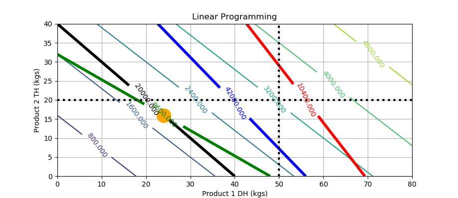
Gekko需要相同数量的变量和约束来执行灵敏度分析。它只适用于正方形系统，在那里你试图理解模型的输入和输出之间的关系。也许您需要的是约束的影子价格，而不是灵敏度分析。因为您的问题只有两个变量，所以您可以使用等高线图来可视化约束和目标。

​

​

from gekko import GEKKO
model = GEKKO(remote=False)
model.options.SENSITIVITY = 0   # sensitivity analysis
model.options.SOLVER = 1        # change solver (1=APOPT,3=IPOPT)
#Maximum demand and implicit contraints as upper bound and lower bound
x1 = model.Var(lb=0, ub=50) # Product DH
x2 = model.Var(lb=0, ub=20) # Product TH
#Objective function
model.Maximize(45*x1+50*x2) # Profit function
#Constraints
model.Equation(500*x1+500*x2<=20000) #Cornflour
model.Equation(750*x1+625*x2<=42000) #Sugar
model.Equation(150*x1+100*x2<=10400) #Fruit and Nut
model.Equation(200*x1+300*x2<=9600) #Ghee
model.solve(disp=True, debug = 1)
p1 = x1.value[0]; p2 = x2.value[0]
print ('Product 1 (DH) in Kgs: ' + str(p1))
print ('Product 2 (TH) in Kgs: ' + str(p2))
print ('Profit       : Rs.' + str(45*p1+50*p2))
print(model.path)


## Generate a contour plot
# Import some other libraries that we'll need
# matplotlib and numpy packages must also be installed
import matplotlib
import numpy as np
import matplotlib.pyplot as plt

# Design variables at mesh points
x1 = np.arange(0.0, 81.0, 2.0)
x2 = np.arange(0.0, 41.0, 2.0)
x1, x2 = np.meshgrid(x1,x2)

# Equations and Constraints
cf = 500*x1+500*x2
sg = 750*x1+625*x2
fn = 150*x1+100*x2
gh = 200*x1+300*x2

# Objective
obj = 45*x1+50*x2

# Create a contour plot
plt.figure()
# Weight contours
CS = plt.contour(x1,x2,obj)
plt.clabel(CS, inline=1, fontsize=10)
# Constraints
CS = plt.contour(x1, x2, cf,[20000],colors='k',linewidths=[4.0])
plt.clabel(CS, inline=1, fontsize=10)
CS = plt.contour(x1, x2, sg,[42000],colors='b',linewidths=[4.0])
plt.clabel(CS, inline=1, fontsize=10)
CS = plt.contour(x1, x2, fn,[10400],colors='r',linewidths=[4.0])
plt.clabel(CS, inline=1, fontsize=10)
CS = plt.contour(x1, x2, gh,[9600],colors='g',linewidths=[4.0])
plt.clabel(CS, inline=1, fontsize=10)

# plot optimal solution
plt.plot(p1,p2,'o',color='orange',markersize=20)

# plot bounds
plt.plot([0,80],[20,20],'k:',lw=3)
plt.plot([50,50],[0,40],'k:',lw=3)

# Add some labels
plt.title('Linear Programming')
plt.xlabel('Product 1 DH (kgs)')
plt.ylabel('Product 2 TH (kgs)')
plt.grid()
plt.savefig('contour.png')
plt.show()

编辑:检索影子价格(拉格朗日乘数)

拉格朗日乘数(影子价格)可用于约束时，您使用IPOPT求解器。将m.options.SOLVER=3设置为IPOPT，并将诊断级别设置为2+和m.options.DIAGLEVEL=2。下面是用于生成影子价格的修改代码：

from gekko import GEKKO
model = GEKKO(remote=False)
model.options.DIAGLEVEL = 2
model.options.SOLVER = 3        # change solver (1=APOPT,3=IPOPT)
#Maximum demand and implicit contraints as upper bound and lower bound
x1 = model.Var(lb=0, ub=50) # Product DH
x2 = model.Var(lb=0, ub=20) # Product TH
#Objective function
model.Maximize(45*x1+50*x2) # Profit function
#Constraints
model.Equation(500*x1+500*x2<=20000) #Cornflour
model.Equation(750*x1+625*x2<=42000) #Sugar
model.Equation(150*x1+100*x2<=10400) #Fruit and Nut
model.Equation(200*x1+300*x2<=9600) #Ghee
model.solve(disp=True, debug = 1)
p1 = x1.value[0]; p2 = x2.value[0]
print ('Product 1 (DH) in Kgs: ' + str(p1))
print ('Product 2 (TH) in Kgs: ' + str(p2))
print ('Profit       : Rs.' + str(45*p1+50*p2))

# for shadow prices, turn on DIAGLEVEL to 2+
#   and use IPOPT solver (APOPT doesn't export Lagrange multipliers)

# Option 1: open the run folder and open apm_lam.txt
model.open_folder()

# Option 2: read apm_lam.txt into array
import numpy as np
lam = np.loadtxt(model.path+'/apm_lam.txt')
print(lam)

结果是：

Product 1 (DH) in Kgs: 24.0
Product 2 (TH) in Kgs: 16.0
Profit       : Rs.1880.0
[-6.99999e-02 -3.44580e-11 -1.01262e-10 -5.00000e-02]