包含交互作用的GLM中的相对重要性/变异分区

Question

在包含交互(连续*因子)的GLM中，我有一个关于变量的相对重要性的问题。

我正在试验一种基于的方法，通过(伪)-R-平方来近似地划分被解释的变化.但我不知道如何在GLM中实现(1)，以及(2)包含交互作用的模型。

为了简单起见，我准备了一个带有一个带有单个交互的Guassian的示例模型(使用mtcar数据集，请参阅文章末尾的代码)。但实际上，我有兴趣将该方法应用于广义Poisson GLM，它可能包含多个相互作用。在测试模型中出现了一些问题：

1. How来正确地划分R-平方？我尝试过一个分区，但我不确定是否正确，每个术语的r-平方加起来不等于整个模型的r-平方(甚至不接近)。，这也发生在不包含交互作用的模型中。除了划分r-平方的错误(我仍然认为自己是统计数据的新手:P)；这是否也会受到共线性的影响？连续预测因子的方差通货膨胀因子在3以下(无标度的模型VIF值最高，为5.7)。

任何帮助都会得到极大的重视！

library(tidyverse)
library(rsq)
library(car)

data <- mtcars %>%
  # scale reduces collinearity: without standardizing, the variance inflation factor for the factor is 5.7
  mutate(disp = scale(disp))
data$am <- factor(data$am)

summary(data)

# test model, continuous response (miles per gallon), type of transmission (automatic/manual) as factor, displacement as continuous
model <-
  glm(mpg ~ am + disp + am:disp,
      data = data,
      family = gaussian(link = "identity"))
drop1(model, test = "F")

# graph the data
ggplot(data = data, aes(x = disp, y = mpg, col = am)) + geom_jitter() + geom_smooth(method = "glm")

# Attempted partitioning
(rsq_full <- rsq::rsq(model, adj = TRUE, type = "v"))

(rsq_int <- rsq_full - rsq::rsq(update(model, . ~ . - am:disp), adj = TRUE, type = "v"))

(rsq_factor <- rsq_full - rsq::rsq(update(model, . ~ . - am - am:disp), adj = TRUE, type = "v"))

(rsq_cont <- rsq_full - rsq::rsq(update(model, . ~ . - disp - am:disp), adj = TRUE, type = "v"))

c(rsq_full, rsq_int + rsq_factor + rsq_cont)

car::vif(model)


# A simpler model with no interaction
model2 <- glm(mpg ~ am + disp, data = data, family = gaussian(link = "identity"))
drop1(model2, test = "F")

(rsq_full2 <- rsq::rsq(model2, adj = TRUE, type = "v"))
(rsq_factor2 <- rsq_full2 - rsq::rsq(update(model2, . ~ . - am), adj = TRUE, type = "v"))
(rsq_cont2 <- rsq_full2 - rsq::rsq(update(model2, . ~ . - disp), adj = TRUE,type = "v"))

c(rsq_full2, rsq_factor2 + rsq_cont2)

car::vif(model2)

Answer 1

给予：

1. y = A + B + A * B

我会比较它的R平方值和它的更简单的版本：

1. y = A + B
2. y = A
3. y = B

如果没有互动，我想

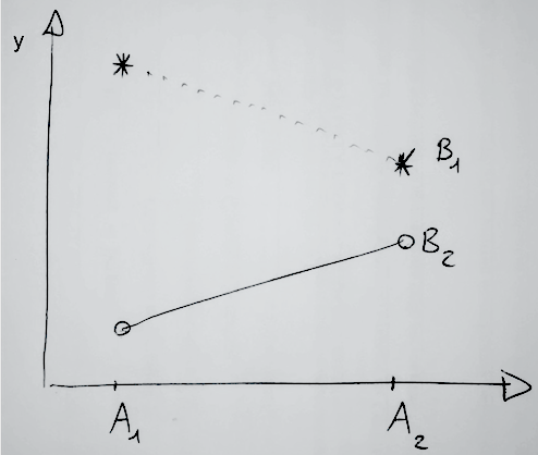
r-squared(model1) = r-squared(model2)

这应该适用于任何线性模型。即使存在相互作用，也应该有助于比较预测因素的主要影响。我知道这是有争议的，但如果您查看下图中表示的场景，预测器A只在考虑到预测器B的情况下才能提供信息；相反，预测器B本身也具有一定的预测能力( B1的y值高于B2的y，而不管它们所属的A级别如何)。

​

​

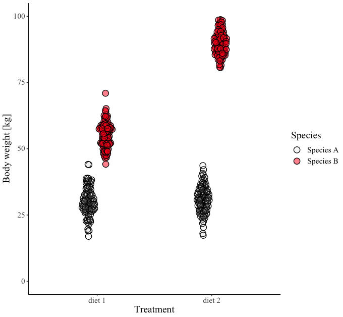
下面是一个模拟数据的例子(为了避免共线性和非正态性问题)：

# simulate data:
df <- data.frame(Species = as.factor(c(rep("Species A", 200),
                            rep("Species B", 200)
                            )),
                Treatment = as.factor(rep(c("diet 1", "diet 2","diet 1", "diet 2"), each=100)),
                body.weight = c(rnorm(n=100, 30, 5),
                                rnorm(n=100, 29.9, 5),
                                rnorm(n=100, 55, 5),
                                rnorm(n=100, 90, 5)
                                )
                )

​

​

# Let's fit and compare the alternative models:
lm.interactive <- lm(body.weight ~ Species * Treatment, data=df)
lm.additive <- lm(body.weight ~ Species + Treatment, data=df)
lm.only.species <- lm(body.weight ~ Species, data=df)
lm.only.Treatment <- lm(body.weight ~ Treatment, data=df)
lm.null <- lm(body.weight ~ 1, data=df)

# obtain R^2:


summary(lm.only.Treatment)$adj.r.squared # main effect of Treatment
summary(lm.only.species)$adj.r.squared # main effect of species ID. 
# As the figure suggests, it's larger than the main effect of Treatment 
# (species identity affects body weight regardless of treatment)
summary(lm.additive)$adj.r.squared # sum of the main effects
summary(lm.interactive)$adj.r.squared # main effects + interaction

# fraction of variance explained by the interaction alone:
summary(lm.interactive)$adj.r.squared - summary(lm.additive)$adj.r.squared

不过，我不确定我们是否真的能谈论“仅由相互作用解释的方差的分数”。说到增加解释的差异，因为纳入了一个相互作用的条件，可能是更合适的。

我不确定我所建议的方法在统计上是否合理，它的局限性，或者它是否对不平衡的数据集可靠地工作。这种方法的一个问题是，对于每个模型，我们只有一个R平方值，因此R平方值的差异不能进行统计检验。一种方法是通过引导获得每个模型的R平方值的分布。