利用gekko优化乙醇生产生物反应器

Question

继续我优化乙醇生物反应器的努力，我开始计划并决定用于帮助我在间歇循环结束时最大限度地提高乙醇浓度的值。这些措施是：

• S0，它是负载型生物反应器中的初始底物浓度。
• Sin，它是生物反应器饲料中的底物浓度，随着时间的推移可能发生变化。
• 秦，这是容积输入法，理想情况下，我想成为一个阶跃函数，以创建一个喂食政策。
• Fc是冷却剂入口容积流量，随着时间的推移可能发生变化，以帮助将生物反应器的温度保持在一定的范围内，以避免由于工作温度高/低而产生的抑制。基本上，它是用来代替温度PID控制器。

当然，批处理时间对于优化我的问题也很重要，但是已经足够复杂了，我暂时忽略它，给它一个固定的值(40小时)。以防万一，我想知道gekko能否决定模拟时间。

因此，我使用了两个关键的绩效指标(KPI)来进行有效的操作：

• 生物反应器生产力越高越好
• 操作过程中基片损耗应尽可能接近零。

考虑到所有这些，我修改了下面的固定代码(非常感谢河登仁教授)，但我认为gekko由于问题的刚性而难以找到解决方案。还有什么其他的建议吗？

# Optimization logic:
# Goal is to maximize ethanol concentration by the end of the batch time, keeping certain KPIs within limits.
# Start with loose boundaries on: Prod, Gloss, T and slowly narrow them down.
# Ideal case: Prod>=4, Gloss = 0 and T = 30-32oC throughout the time horizon, for that a PID controller might later be added.
# Manipulated variables to achieve goal are: Qin, Sin, S0, Fc (Vl0 and batch time might as well be added).
# Qin to be a step function, Sin can change to have substrate concentration at different levels in feed, S0 is fixed (concentration of substrate in loaded BR)
# and Fc should be time dependant to ensure T is within boundaries.
# Constraint due to problem definition on bioreactor working volume: Vl=<0.8V

from gekko import GEKKO
import numpy as np
import matplotlib.pyplot as plt


m = GEKKO(remote=False)
# Create time vector [hours]
tm = np.linspace(0,40,401)
# Insert smaller time steps at the beginning
tm = np.insert(tm,1,[0.001,0.005,0.01,0.05])
m.time = tm
nt = len(tm)

# Define constants and parameters
#################################
# Kinetic Parameters
a1     = m.Const(value=0.05, name='a1')     # Ratkowsky parameter [oC-1 h-0.5]
aP     = m.Const(value=4.50, name='aP')     # Growth-associated parameter for EtOh production [-]
AP1    = m.Const(value=6.0, name='AP1')     # Activation energy parameter for EtOh production [oC]
AP2    = m.Const(value=20.3, name='AP2')    # Activation energy parameter for EtOh production [oC]
b1     = m.Const(value=0.035, name='b1')    # Parameter in the exponential expression of the maximum specific growth rate expression [oC-1]
b2     = m.Const(value=0.15, name='b2')     # Parameter in the exponential expression of the maximum specific growth rate expression [oC-1]
b3     = m.Const(value=0.40, name='b3')     # Parameter in the exponential expression of the specific death rate expression [oC-1]
c1     = m.Const(value=0.38, name='c1')     # Constant decoupling factor for EtOh [kgP kgX-1 h-1]
c2     = m.Const(value=0.29, name='c2')     # Constant decoupling factor for EtOh [kgP kgX-1 h-1]
k1     = m.Const(value=3, name='k1')        # Parameter in the maximum specific growth rate expression [oC]
k2     = m.Const(value=55, name='k2')       # Parameter in the maximum specific growth rate expression [oC]
k3     = m.Const(value=60, name='k3')       # Parameter in the growth-inhibitory EtOH concentration expression [oC]
k4     = m.Const(value=50, name='k4')       # Temperature at the inflection point of the specific death rate sigmoid curve [oC]
Pmaxb  = m.Const(value=90, name='Pmaxb')    # Temperature-independent product inhibition constant [kg m-3]
PmaxT  = m.Const(value=90, name='PmaxT')    # Maximum value of product inhibition constant due to temperature [kg m-3]
Kdb    = m.Const(value=0.025, name='Kdb')   # Basal specific cellular biomass death rate [h-1]
KdT    = m.Const(value=30, name='KdT')      # Maximum value of specific cellular biomass death rate due to temperature [h-1]
KSX    = m.Const(value=5, name='KSX')       # Glucose saturation constant for the specific growth rate [kg m-3]
KOX    = m.Const(value=0.0005, name='KOX')  # Oxygen saturation constant for the specific growth rate [kg m-3]
qOmax  = m.Const(value=0.05, name='qOmax')  # Maximum specific oxygen consumption rate [h-1]

# Metabolic Parameters
YPS    = m.Const(value=0.51, name='YPS')    # Theoretical yield of EtOH on glucose [kgP kgS-1]
YXO    = m.Const(value=0.97, name='YXO')    # Theoretical yield of biomass on oxygen [kgX kgO-1]
YXS    = m.Const(value=0.53, name='YXS')    # Theoretical yield of biomass on glucose [kgX kgS-1]

# Physicochemical and thermodynamic parameters
Chbr   = m.Const(value=4.18, name='Chbr')      # Heat capacity of the mass of reaction [kJ kg-1 oC-1]
Chc    = m.Const(value=4.18, name='Chc')       # Heat capacity of cooling agent [kJ kg-1 oC-1]
deltaH = m.Const(value=518.e3, name='deltaH')  # Heat of reaction of fermentation [kJ kmol-1 O2]
Tref   = m.Const(value=25, name='Tref')        # Reference temperature [oC]
KH     = m.Const(value=200, name='KH')         # Henry's constant for oxygen in the fermentation broth [atm m3 kmol-1]
z      = m.Const(value=0.792, name='z')        # Oxygen compressibility factor [-]
R      = m.Const(value=0.082, name='R')        # Ideal gas constant [m3 atm kmol-1 oC-1]
kla0   = m.Const(value=100, name='kla0')       # Temperature-independent volumetric oxygen transfer coefficient [-h]
KT     = m.Const(value=360, name='KT')         # Heat transfer coefficient [kJ h-1 m-2 oC-1]
rho    = m.Const(value=1080, name='rho')       # Density of the fermentation broth [kg m-3]
rhoc   = m.Const(value=1000, name='rhoc')      # Density of the cooling agent [kg m-3]
MO     = m.Const(value=31.998, name='MO')      # Molecular weight of oxygen [kg kmol-1]

# Bioreactor design data
AT     = m.Const(value=100, name='AT')        # Bioreactor heat transfer area [m2]
V      = m.Const(value=2900, name='V')        # Bioreactor working volume [m3]
Vcj    = m.Const(value=250, name='Vcj')       # Cooling jacket volume [m3]
Ogasin = m.Const(value=0.305, name='Ogasin')  # Oxygen concentration in airflow inlet [kg m-3]

# Define variables
##################
# Manipulated Variables
S0 = m.FV(value=50, lb=+0.0, ub=10000, name='S0')  # Initial substrate concentration in loaded bioreactor [kg m-3]
S0.STATUS = 1

Sin = m.MV(value=400, lb=0, ub=1500)  # Substrate/Glucose concentration in bioreactor feed [kg m-3]
Sin.STATUS = 1
Sin.DCOST = 0.0

Qin = m.MV(value=0, name='Qin')  # Ideally Qin to be a step function
Qin.STATUS = 1
Qin.DCOST = 0.0

Fc  = m.FV(value=40, name='Fc')  # Coolant inlet volumetric flow rate [m3 h-1]
Fc.STATUS = 1

# Variables
mi = m.Var(name='mi', lb=0)  # Specific growth rate [kgP kgX-1 h-1]
bP = m.Var(name='bP', lb=0)  # Non-growth associated term [kgP kgX-1 h-1]

# KPIs variables
XXt   = m.Var(name='XXt')              # Biomass yield of glucose fermentation
XP    = m.Var(name='XP')               # Ethanol yield of glucose fermentation
Prod  = m.Var(name='Prod', lb=1)       # Bioreactor productivity in ethanol
Gloss = m.Var(name='Gloss', ub=10000)  # Substrate loss during fed-batch operation

# Fixed variables, they are constant throughout the time horizon
Xtin = m.FV(value=0, name='Xtin')      # Total cellular biomass concentration in the bioreactor feed [kg/m3]
Xvin = m.FV(value=0, name='Xvin')      # Viable cellular biomass concentration in the bioreactor feed [kg/m3]
Qe   = m.FV(value=0, name='Qe')        # Output flow rate [m3/h]
Pin  = m.FV(value=0, name='Pin')       # Ethanol concentration in the bioreactor feed [kg/m3]
Fair = m.FV(value=60000, name='Fair')  # Air flow volumetric rate [m3/h]
Tin  = m.FV(value=30, name='Tin')      # Temperature of bioreactor feed [oC]
Tcin = m.FV(value=15, name='Tcin')     # Temperature of coolant inlet [oC]

# Differential equations variables
Vl     = m.Var(value=1000, ub=0.8*V, name='Vl')   # [m3]
Xt     = m.Var(value=0.1, name='Xt')              # [kg m-3]
Xv     = m.Var(value=0.1, name='Xv')              # [kg m-3]
S      = m.Var(value=S0, name='S')                # [kg m-3]
P      = m.Var(value=0, name='P')                 # [kg m-3]
Ol     = m.Var(value=0.0065, name= 'Ol')          # [kg m-3]
Og     = m.Var(value=0.305, name='Og')            # [kg m-3]
T      = m.Var(value=30, lb=20, ub=40, name='T')  # [oC]
Tc     = m.Var(value=20, name='Tc')               # [oC]
Sf_cum = m.Var(value=0, name='Sf_cum')            # [kg]
t      = m.Var(value=0, name='Time')              # [h]

# Define algebraic equations
############################
# Specific growth rate of cell mass
mimax = m.Intermediate(((a1*(T-k1))*(1-m.exp(b1*(T-k2)))) ** 2)
Pmax  = m.Intermediate(Pmaxb + PmaxT/(1-m.exp(-b2*(T-k3))))
m.Equation(mi == mimax * S/(KSX+S) * Ol/(KOX + Ol) * (1 - P/Pmax) * 1 / (1+m.exp(-(100-S)/1)))
# Specific production rate of EtOH
m.Equation(bP == c1*m.exp(-AP1/T) - c2*m.exp(-AP2/T))
qP    = m.Intermediate(aP*mi + bP)
# Specific consumption rate of glucose
qS    = m.Intermediate(mi/YXS + qP/YPS)
# Specific consumption rate of oxygen
qO    = m.Intermediate(qOmax*Ol/YXO/(KOX+Ol))
# Specific biological deactivation rate of cell mass
Kd    = m.Intermediate(Kdb + KdT/(1+m.exp(-b3*(T-k4))))
# Saturation concentration of oxygen in culture media
Ostar = m.Intermediate(z*Og*R*T/KH)
# Oxygen mass transfer coefficient
kla   = m.Intermediate(kla0*1.2**(T-20))
# Bioreactor phases equation
Vg    = m.Intermediate(V - Vl)

# Define differential equations
###############################
m.Equation(Vl.dt()     == Qin - Qe)
m.Equation(Vl*Xt.dt()  == Qin*(Xtin-Xt) + mi*Vl*Xv)
m.Equation(Vl*Xv.dt()  == Qin*(Xvin-Xv) + Xv*Vl*(mi-Kd))
m.Equation(Vl*S.dt()   == Qin*(Sin-S) - qS*Vl*Xv)
m.Equation(Vl*P.dt()   == Qin*(Pin-P) + qP*Vl*Xv)
m.Equation(Vl*Ol.dt()  == Qin*(Ostar-Ol)  + Vl*kla*(Ostar-Ol) - qO*Vl*Xv)
m.Equation(Vg*Og.dt()  == Fair*(Ogasin-Og) - Vl*kla*(Ostar-Ol) + Og*(Qin-Qe))
m.Equation(Vl*T.dt()   == Qin*(Tin-T) - Tref*(Qin-Qe) + Vl*qO*Xv*deltaH/MO/rho/Chbr - KT*AT*(T-Tc)/rho/Chbr)
m.Equation(Vcj*Tc.dt() == Fc*(Tcin - Tc) + KT*AT*(T-Tc)/rhoc/Chc)
m.Equation(Sf_cum.dt() == Qin*Sin)
m.Equation(t.dt()      == 1)

# Yields and Productivity
#########################
m.Equation(XXt   == (Xt*Vl - Xt.value*Vl.value)/(S.value*Vl.value + Sf_cum))
m.Equation(XP    == (P*Vl - P.value*Vl.value)/(S.value*Vl.value + Sf_cum))
m.Equation(Prod  == (P-P.value)/t)
m.Equation(Gloss == Vl*S)

# solve DAE
m.options.SOLVER= 1
m.options.IMODE = 7
m.options.NODES = 3
m.options.MAX_ITER = 3000
# m.open_folder()
m.solve()

# Objective function
f = np.zeros(nt)
f[-1] = 1.0
final = m.Param(value=f)
m.Obj(-final*P)

# Solve optimization problem
m.options.IMODE=6
m.solve()

print('Total loss of substrate: G=' + str(Gloss.value[-1]) + '[kg]')
print('Biomass: Xt=' + str(Xt.value[-1]) + '[kg/m3]')
print('Ethanol: P=' + str(P.value[-1])  + '[kg/m3]')
print('Bioreactor productivity: Prod=' + str(Prod.value[-1])  + '[kg/m3/h]')
print('Bioreactor operating volume: Vl='+ str(Vl.value[-1]) + '[m3]')

# Plot results
plt.figure(0)
plt.title('Feeding Policy')
plt.plot(m.time, Qin.value, label='Qin')
plt.ylabel('Qin [m3/h]')
plt.xlabel('Time [h]')
plt.legend(); plt.grid(); plt.minorticks_on()
plt.ylim(0); plt.xlim(m.time[0],m.time[-1])
plt.tight_layout()

plt.figure(1)
plt.title('Total & Viable Cellular Biomass')
plt.plot(m.time, Xv.value, label='Xv')
plt.plot(m.time, Xt.value, label='Xt')
plt.ylabel('Biomass concentration [kg/m3]')
plt.xlabel('Time [h]')
plt.legend(); plt.grid(); plt.minorticks_on()
plt.ylim(0); plt.xlim(m.time[0],m.time[-1])
plt.tight_layout()

plt.figure(2)
plt.title('Substrate (S) & Product (P) concentration')
plt.plot(m.time, S.value, label='S')
plt.plot(m.time, P.value, label='P')
plt.ylabel('Concentration [kg/m3]')
plt.xlabel('Time [h]')
plt.legend(); plt.grid(); plt.minorticks_on()
plt.ylim(0); plt.xlim(m.time[0],m.time[-1])
plt.tight_layout()

fig3, ax = plt.subplots()
ax.title.set_text('Dissolved & Gaseous Oxygen concentration')
lns1 = ax.plot(m.time, Ol.value, label='[Oliq]', color='c')
ax.set_xlabel('Time [h]')
ax.set_ylabel('Oliq [kg/m3]', color='c')
ax.minorticks_on()
ax2 = ax.twinx()
lns2 = ax2.plot(m.time, Og.value, label='[Ogas]', color='y')
ax2.set_ylabel('Ogas [kg/m3]', color='y')
ax2.minorticks_on()
lns = lns1 + lns2
labs = [l.get_label() for l in lns]
ax.legend(lns, labs, loc='best')
ax.grid()
ax.set_xlim(m.time[0],m.time[-1])
fig3.tight_layout()
plt.figure(3)

plt.figure(4)
plt.title('Bioreactor & Cooling jacket temperature')
plt.plot(m.time, T.value, label='T')
plt.plot(m.time, Tc.value, label='Tc')
plt.ylabel('Temperature [oC]')
plt.xlabel('Time [h]')
plt.legend(); plt.grid(); plt.minorticks_on()
plt.ylim(0); plt.xlim(m.time[0],m.time[-1])
plt.tight_layout()

fig5, ax = plt.subplots()
ax.title.set_text('Specific rates & bP')
lns1 = ax.plot(tm,Kd.value,label='Kd')
lns2 = ax.plot(tm,mimax.value,label='mimax')
lns3 = ax.plot(tm,mi.value,label='mi')
ax.set_xlabel('Time [h]')
ax.set_ylabel('Specific growth and death rate')
ax.minorticks_on()
ax2 = ax.twinx()
lns4 = ax.plot(tm,bP.value,label='bP', color='magenta')
ax2.set_ylabel('bP [1/h]', color='magenta')
ax2.minorticks_on()
lns = lns1 + lns2 + lns3 + lns4
labs = [l.get_label() for l in lns]
ax.legend(lns, labs, loc='best'); ax.grid()
ax.set_ylim(0); ax.set_xlim(m.time[0],m.time[-1])
fig5.tight_layout()
plt.figure(5)

fig6, ax = plt.subplots()
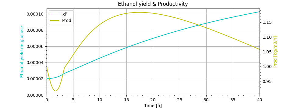
ax.title.set_text('Ethanol yield & Productivity')
lns1 = ax.plot(m.time, XP.value, label='xP', color='c')
ax.set_xlabel('Time [h]')
ax.set_ylabel('Ethanol yield on glucose', color='c')
ax.minorticks_on()
ax2 = ax.twinx()
lns2 = ax2.plot(m.time, Prod.value, label='Prod', color='y')
ax2.set_ylabel('Prod [kg/m3/h]', color='y')
ax2.minorticks_on()
lns = lns1 + lns2
labs = [l.get_label() for l in lns]
ax.legend(lns, labs, loc='best')
ax.grid()
ax.set_ylim(0); ax.set_xlim(m.time[0],m.time[-1])
fig6.tight_layout()
plt.figure(6)

fig7, ax = plt.subplots()
ax.title.set_text('Culture Volume & Total Substrate fed to the Bioreactor')
lns1 = ax.plot(m.time, Vl.value, label='Vl', color='r')
ax.set_xlabel('Time [h]')
ax.set_ylabel('Vl [m3]', color='r')
ax.minorticks_on()
ax2 = ax.twinx()
lns2 = ax2.plot(m.time, Sf_cum.value, label='Sf_cum', color='g')
ax2.set_ylabel('Sf_cum [kg]', color='g')
ax2.minorticks_on()
lns = lns1 + lns2
labs = [l.get_label() for l in lns]
ax.legend(lns, labs, loc='best')
ax.grid()
ax.set_ylim(900); ax2.set_ylim(0); ax.set_xlim(m.time[0],m.time[-1])
fig7.tight_layout()
plt.figure(7)

plt.show()

Answer 1

以下是一些建议：

• 重新排列方程以避免被除以零
• KPI方程不影响其他变量，可以在求解后转换为中间变量或进行计算。
• 使用COLDSTART和2..1.0分别对模型进行初始化
• 在模拟初始化(COLDSTART=2,1)之后添加约束。这些约束使得仿真变得不可行。
• 向决策变量(如Qin )添加上界和下界。
• 使用m.free_initial(S)计算初始条件S0。我暂时忘了这个，但你可以把它加回去。
• 使用MV_STEP_HOR=100将Qin或Sin的更改次数减少到每批4次，以减少操作员操作。
• (可选)考虑固定温度，以优化产量，并假设有一个较低级别控制器的优秀温度控制。这将消除能量平衡方程，以后可以添加。它还将有助于提高求解速度，并消除模型中一些具有挑战性的速率方程指数项。
• (可选)切换到公共服务器(remote=True)，查看迭代摘要并监视解决程序的进度。本地模式目前没有这种能力。

下面是经过30次迭代后几乎成功解决的代码。它可能需要一些额外的调整，例如COLDSTART=0的约束，以获得解决方案和您期望的结果。

​

​

# Optimization logic:
# Goal is to maximize ethanol concentration by the end of the batch time, keeping certain KPIs within limits.
# Start with loose boundaries on: Prod, Gloss, T and slowly narrow them down.
# Ideal case: Prod>=4, Gloss = 0 and T = 30-32oC throughout the time horizon, for that a PID controller might later be added.
# Manipulated variables to achieve goal are: Qin, Sin, S0, Fc (Vl0 and batch time might as well be added).
# Qin to be a step function, Sin can change to have substrate concentration at different levels in feed, S0 is fixed (concentration of substrate in loaded BR)
# and Fc should be time dependant to ensure T is within boundaries.
# Constraint due to problem definition on bioreactor working volume: Vl=<0.8V

from gekko import GEKKO
import numpy as np
import matplotlib.pyplot as plt


m = GEKKO(remote=True)
# Create time vector [hours]
tm = np.linspace(0,40,401)
# Insert smaller time steps at the beginning
tm = np.insert(tm,1,[0.001,0.005,0.01,0.05])
m.time = tm
nt = len(tm)

# Define constants and parameters
#################################
# Kinetic Parameters
a1     = m.Const(value=0.05, name='a1')     # Ratkowsky parameter [oC-1 h-0.5]
aP     = m.Const(value=4.50, name='aP')     # Growth-associated parameter for EtOh production [-]
AP1    = m.Const(value=6.0, name='AP1')     # Activation energy parameter for EtOh production [oC]
AP2    = m.Const(value=20.3, name='AP2')    # Activation energy parameter for EtOh production [oC]
b1     = m.Const(value=0.035, name='b1')    # Parameter in the exponential expression of the maximum specific growth rate expression [oC-1]
b2     = m.Const(value=0.15, name='b2')     # Parameter in the exponential expression of the maximum specific growth rate expression [oC-1]
b3     = m.Const(value=0.40, name='b3')     # Parameter in the exponential expression of the specific death rate expression [oC-1]
c1     = m.Const(value=0.38, name='c1')     # Constant decoupling factor for EtOh [kgP kgX-1 h-1]
c2     = m.Const(value=0.29, name='c2')     # Constant decoupling factor for EtOh [kgP kgX-1 h-1]
k1     = m.Const(value=3, name='k1')        # Parameter in the maximum specific growth rate expression [oC]
k2     = m.Const(value=55, name='k2')       # Parameter in the maximum specific growth rate expression [oC]
k3     = m.Const(value=60, name='k3')       # Parameter in the growth-inhibitory EtOH concentration expression [oC]
k4     = m.Const(value=50, name='k4')       # Temperature at the inflection point of the specific death rate sigmoid curve [oC]
Pmaxb  = m.Const(value=90, name='Pmaxb')    # Temperature-independent product inhibition constant [kg m-3]
PmaxT  = m.Const(value=90, name='PmaxT')    # Maximum value of product inhibition constant due to temperature [kg m-3]
Kdb    = m.Const(value=0.025, name='Kdb')   # Basal specific cellular biomass death rate [h-1]
KdT    = m.Const(value=30, name='KdT')      # Maximum value of specific cellular biomass death rate due to temperature [h-1]
KSX    = m.Const(value=5, name='KSX')       # Glucose saturation constant for the specific growth rate [kg m-3]
KOX    = m.Const(value=0.0005, name='KOX')  # Oxygen saturation constant for the specific growth rate [kg m-3]
qOmax  = m.Const(value=0.05, name='qOmax')  # Maximum specific oxygen consumption rate [h-1]

# Metabolic Parameters
YPS    = m.Const(value=0.51, name='YPS')    # Theoretical yield of EtOH on glucose [kgP kgS-1]
YXO    = m.Const(value=0.97, name='YXO')    # Theoretical yield of biomass on oxygen [kgX kgO-1]
YXS    = m.Const(value=0.53, name='YXS')    # Theoretical yield of biomass on glucose [kgX kgS-1]

# Physicochemical and thermodynamic parameters
Chbr   = m.Const(value=4.18, name='Chbr')      # Heat capacity of the mass of reaction [kJ kg-1 oC-1]
Chc    = m.Const(value=4.18, name='Chc')       # Heat capacity of cooling agent [kJ kg-1 oC-1]
deltaH = m.Const(value=518.e3, name='deltaH')  # Heat of reaction of fermentation [kJ kmol-1 O2]
Tref   = m.Const(value=25, name='Tref')        # Reference temperature [oC]
KH     = m.Const(value=200, name='KH')         # Henry's constant for oxygen in the fermentation broth [atm m3 kmol-1]
z      = m.Const(value=0.792, name='z')        # Oxygen compressibility factor [-]
R      = m.Const(value=0.082, name='R')        # Ideal gas constant [m3 atm kmol-1 oC-1]
kla0   = m.Const(value=100, name='kla0')       # Temperature-independent volumetric oxygen transfer coefficient [-h]
KT     = m.Const(value=360, name='KT')         # Heat transfer coefficient [kJ h-1 m-2 oC-1]
rho    = m.Const(value=1080, name='rho')       # Density of the fermentation broth [kg m-3]
rhoc   = m.Const(value=1000, name='rhoc')      # Density of the cooling agent [kg m-3]
MO     = m.Const(value=31.998, name='MO')      # Molecular weight of oxygen [kg kmol-1]

# Bioreactor design data
AT     = m.Const(value=100, name='AT')        # Bioreactor heat transfer area [m2]
V      = m.Const(value=2900, name='V')        # Bioreactor working volume [m3]
Vcj    = m.Const(value=250, name='Vcj')       # Cooling jacket volume [m3]
Ogasin = m.Const(value=0.305, name='Ogasin')  # Oxygen concentration in airflow inlet [kg m-3]

# Define variables
##################
# Manipulated Variables
#S0 = m.FV(value=50, lb=+0.0, ub=10000, name='S0')  # Initial substrate concentration in loaded bioreactor [kg m-3]
#S0.STATUS = 1
# use m.free_initial(S) after initialization

Sin = m.MV(value=400, lb=0, ub=1500)  # Substrate/Glucose concentration in bioreactor feed [kg m-3]
Sin.STATUS = 1
Sin.DCOST = 0.0
Sin.MV_STEP_HOR = 100

Qin = m.MV(value=0.1, lb=0.1, ub=100, name='Qin')  # Ideally Qin to be a step function
Qin.STATUS = 1
Qin.DCOST = 0.0
Qin.MV_STEP_HOR = 100

Fc  = m.FV(value=40, lb=0, ub=1e4, name='Fc')  # Coolant inlet volumetric flow rate [m3 h-1]
Fc.STATUS = 1

# Variables
mi = m.Var(name='mi')  # Specific growth rate [kgP kgX-1 h-1]
bP = m.Var(name='bP')  # Non-growth associated term [kgP kgX-1 h-1]

# Fixed variables, they are constant throughout the time horizon
Xtin = m.FV(value=0, name='Xtin')      # Total cellular biomass concentration in the bioreactor feed [kg/m3]
Xvin = m.FV(value=0, name='Xvin')      # Viable cellular biomass concentration in the bioreactor feed [kg/m3]
Qe   = m.FV(value=0, name='Qe')        # Output flow rate [m3/h]
Pin  = m.FV(value=0, name='Pin')       # Ethanol concentration in the bioreactor feed [kg/m3]
Fair = m.FV(value=60000, name='Fair')  # Air flow volumetric rate [m3/h]
Tin  = m.FV(value=30, name='Tin')      # Temperature of bioreactor feed [oC]
Tcin = m.FV(value=15, name='Tcin')     # Temperature of coolant inlet [oC]

# Differential equations variables
Vl0 = 1000; Xt0 = 0.1; P0 = 0; S0 = 50
Vl     = m.Var(value=Vl0, name='Vl')              # [m3]
Xt     = m.Var(value=Xt0, name='Xt')              # [kg m-3]
Xv     = m.Var(value=0.1, name='Xv')              # [kg m-3]
S      = m.Var(value=S0, name='S')                # [kg m-3]
P      = m.Var(value=P0, name='P')                # [kg m-3]
Ol     = m.Var(value=0.0065, name= 'Ol')          # [kg m-3]
Og     = m.Var(value=0.305, name='Og')            # [kg m-3]
T      = m.Var(value=30,name='T')                 # [oC]
Tc     = m.Var(value=20, name='Tc')               # [oC]
Sf_cum = m.Var(value=0, name='Sf_cum')            # [kg]

# Define algebraic equations
############################
# Specific growth rate of cell mass
mimax = m.Intermediate(((a1*(T-k1))*(1-m.exp(b1*(T-k2)))) ** 2)
Pmax  = m.Intermediate(Pmaxb + PmaxT/(1-m.exp(-b2*(T-k3))))
m.Equation(mi == mimax * S/(KSX+S) * Ol/(KOX + Ol) * (1 - P/Pmax) * 1 / (1+m.exp(-(100-S)/1)))
# Specific production rate of EtOH
bPe = m.Intermediate(c1*m.exp(-AP1/T) - c2*m.exp(-AP2/T))
m.Equation(bP == bPe)
qP    = m.Intermediate(aP*mi + bP)
# Specific consumption rate of glucose
qS    = m.Intermediate(mi/YXS + qP/YPS)
# Specific consumption rate of oxygen
qO    = m.Intermediate(qOmax*Ol/YXO/(KOX+Ol))
# Specific biological deactivation rate of cell mass
Kd    = m.Intermediate(Kdb + KdT/(1+m.exp(-b3*(T-k4))))
# Saturation concentration of oxygen in culture media
Ostar = m.Intermediate(z*Og*R*T/KH)
# Oxygen mass transfer coefficient
kla   = m.Intermediate(kla0*1.2**(T-20))
# Bioreactor phases equation
Vg    = m.Intermediate(V - Vl)

# Define differential equations
###############################
m.Equation(Vl.dt()     == Qin - Qe)
m.Equation(Vl*Xt.dt()  == Qin*(Xtin-Xt) + mi*Vl*Xv)
m.Equation(Vl*Xv.dt()  == Qin*(Xvin-Xv) + Xv*Vl*(mi-Kd))
m.Equation(Vl*S.dt()   == Qin*(Sin-S) - qS*Vl*Xv)
m.Equation(Vl*P.dt()   == Qin*(Pin-P) + qP*Vl*Xv)
m.Equation(Vl*Ol.dt()  == Qin*(Ostar-Ol)  + Vl*kla*(Ostar-Ol) - qO*Vl*Xv)
m.Equation(Vg*Og.dt()  == Fair*(Ogasin-Og) - Vl*kla*(Ostar-Ol) + Og*(Qin-Qe))
m.Equation(Vl*T.dt()   == Qin*(Tin-T) - Tref*(Qin-Qe) + Vl*qO*Xv*deltaH/MO/rho/Chbr - KT*AT*(T-Tc)/rho/Chbr)
m.Equation(Vcj*Tc.dt() == Fc*(Tcin - Tc) + KT*AT*(T-Tc)/rhoc/Chc)
m.Equation(Sf_cum.dt() == Qin*Sin)

# KPIs as Intermediates or Var/Equations
kpi_interm = True
if kpi_interm:
    t     = m.Param(m.time)
    XXt   = m.Intermediate((Xt*Vl - Xt0*Vl0)/(S0*Vl0 + Sf_cum))
    XP    = m.Intermediate((P*Vl - P0*Vl0)/(S0*Vl0 + Sf_cum))
    Prod  = m.Intermediate((P-P0)/t)
    Gloss = m.Intermediate(Vl*S)
else:
    # include KPIs as equations
    # KPIs variables
    t      = m.Var(value=0, name='Time')              # [h]
    XXt   = m.Var(name='XXt')              # Biomass yield of glucose fermentation
    XP    = m.Var(name='XP')               # Ethanol yield of glucose fermentation
    Prod  = m.Var(name='Prod') #, lb=1)       # Bioreactor productivity in ethanol
    Gloss = m.Var(name='Gloss')  # Substrate loss during fed-batch operation

    # Yields and Productivity
    #########################
    m.Equation(t.dt()      == 1)
    m.Equation(XXt*(S0*Vl0 + Sf_cum) == (Xt*Vl - Xt0*Vl0))
    m.Equation(XP *(S0*Vl0 + Sf_cum) == (P*Vl - P0*Vl0))
    m.Equation(Prod * t  == (P-P0))
    m.Equation(Gloss == Vl*S)

mi.LOWER = 0
bP.LOWER = 0
T.LOWER=0

# solve DAE
m.options.SOLVER= 1
m.options.REDUCE = 3
m.options.NODES = 2
m.options.IMODE = 6
m.options.COLDSTART = 2
m.options.MAX_ITER = 3000
# m.open_folder()
print('Start Coldstart Simulation')
m.solve()
print('End Coldstart Simulation')

# Objective function
f = np.zeros(nt)
f[-1] = 1.0
final = m.Param(value=f)
m.Maximize(final*P)

# Solve optimization problem
#m.options.SOLVER = 3
m.options.TIME_SHIFT = 0
m.options.COLDSTART=1
m.options.NODES=3
m.options.IMODE=6
print('Start Optimization Coldstart')
m.solve(disp=True)
print('End Optimization Coldstart')

# Add some variable bounds back after simulation
T.UPPER=40
P.LOWER = 0
Gloss.UPPER=10000
Vl.UPPER=0.8*V 

# Calculate S0
m.free_initial(S)

m.options.TIME_SHIFT=0
m.options.COLDSTART=0
m.options.NODES=3
m.options.IMODE=6
m.options.SOLVER= 1
print('Start Optimization')
m.solve(disp=True)
print('End Optimization')

print('Total loss of substrate: G=' + str(Gloss.value[-1]) + '[kg]')
print('Biomass: Xt=' + str(Xt.value[-1]) + '[kg/m3]')
print('Ethanol: P=' + str(P.value[-1])  + '[kg/m3]')
print('Bioreactor productivity: Prod=' + str(Prod.value[-1])  + '[kg/m3/h]')
print('Bioreactor operating volume: Vl='+ str(Vl.value[-1]) + '[m3]')

# Plot results
plt.figure(0)
plt.title('Feeding Policy')
plt.plot(m.time, Qin.value, label='Qin')
plt.ylabel('Qin [m3/h]')
plt.xlabel('Time [h]')
plt.legend(); plt.grid(); plt.minorticks_on()
plt.ylim(0); plt.xlim(m.time[0],m.time[-1])
plt.tight_layout()

plt.figure(1)
plt.title('Total & Viable Cellular Biomass')
plt.plot(m.time, Xv.value, label='Xv')
plt.plot(m.time, Xt.value, label='Xt')
plt.ylabel('Biomass concentration [kg/m3]')
plt.xlabel('Time [h]')
plt.legend(); plt.grid(); plt.minorticks_on()
plt.ylim(0); plt.xlim(m.time[0],m.time[-1])
plt.tight_layout()

plt.figure(2)
plt.title('Substrate (S) & Product (P) concentration')
plt.plot(m.time, S.value, label='S')
plt.plot(m.time, P.value, label='P')
plt.ylabel('Concentration [kg/m3]')
plt.xlabel('Time [h]')
plt.legend(); plt.grid(); plt.minorticks_on()
plt.ylim(0); plt.xlim(m.time[0],m.time[-1])
plt.tight_layout()

fig3, ax = plt.subplots()
ax.title.set_text('Dissolved & Gaseous Oxygen concentration')
lns1 = ax.plot(m.time, Ol.value, label='[Oliq]', color='c')
ax.set_xlabel('Time [h]')
ax.set_ylabel('Oliq [kg/m3]', color='c')
ax.minorticks_on()
ax2 = ax.twinx()
lns2 = ax2.plot(m.time, Og.value, label='[Ogas]', color='y')
ax2.set_ylabel('Ogas [kg/m3]', color='y')
ax2.minorticks_on()
lns = lns1 + lns2
labs = [l.get_label() for l in lns]
ax.legend(lns, labs, loc='best')
ax.grid()
ax.set_xlim(m.time[0],m.time[-1])
fig3.tight_layout()
plt.figure(3)

plt.figure(4)
plt.title('Bioreactor & Cooling jacket temperature')
plt.plot(m.time, T.value, label='T')
plt.plot(m.time, Tc.value, label='Tc')
plt.ylabel('Temperature [oC]')
plt.xlabel('Time [h]')
plt.legend(); plt.grid(); plt.minorticks_on()
plt.ylim(0); plt.xlim(m.time[0],m.time[-1])
plt.tight_layout()

fig5, ax = plt.subplots()
ax.title.set_text('Specific rates & bP')
lns1 = ax.plot(tm,Kd.value,label='Kd')
lns2 = ax.plot(tm,mimax.value,label='mimax')
lns3 = ax.plot(tm,mi.value,label='mi')
ax.set_xlabel('Time [h]')
ax.set_ylabel('Specific growth and death rate')
ax.minorticks_on()
ax2 = ax.twinx()
lns4 = ax.plot(tm,bP.value,label='bP', color='magenta')
ax2.set_ylabel('bP [1/h]', color='magenta')
ax2.minorticks_on()
lns = lns1 + lns2 + lns3 + lns4
labs = [l.get_label() for l in lns]
ax.legend(lns, labs, loc='best'); ax.grid()
ax.set_ylim(0); ax.set_xlim(m.time[0],m.time[-1])
fig5.tight_layout()
plt.figure(5)

fig6, ax = plt.subplots()
ax.title.set_text('Ethanol yield & Productivity')
lns1 = ax.plot(m.time, XP.value, label='xP', color='c')
ax.set_xlabel('Time [h]')
ax.set_ylabel('Ethanol yield on glucose', color='c')
ax.minorticks_on()
ax2 = ax.twinx()
lns2 = ax2.plot(m.time, Prod.value, label='Prod', color='y')
ax2.set_ylabel('Prod [kg/m3/h]', color='y')
ax2.minorticks_on()
lns = lns1 + lns2
labs = [l.get_label() for l in lns]
ax.legend(lns, labs, loc='best')
ax.grid()
ax.set_ylim(0); ax.set_xlim(m.time[0],m.time[-1])
fig6.tight_layout()
plt.figure(6)

fig7, ax = plt.subplots()
ax.title.set_text('Culture Volume & Total Substrate fed to the Bioreactor')
lns1 = ax.plot(m.time, Vl.value, label='Vl', color='r')
ax.set_xlabel('Time [h]')
ax.set_ylabel('Vl [m3]', color='r')
ax.minorticks_on()
ax2 = ax.twinx()
lns2 = ax2.plot(m.time, Sf_cum.value, label='Sf_cum', color='g')
ax2.set_ylabel('Sf_cum [kg]', color='g')
ax2.minorticks_on()
lns = lns1 + lns2
labs = [l.get_label() for l in lns]
ax.legend(lns, labs, loc='best')
ax.grid()
ax.set_ylim(900); ax2.set_ylim(0); ax.set_xlim(m.time[0],m.time[-1])
fig7.tight_layout()
plt.figure(7)

plt.show()

还可以优化整个批处理时间。有关示例，请参见詹宁斯问题。