文章/答案/技术大牛

发布

社区首页 >问答首页 >利用GEKKO生物反应器模拟乙醇生产

问利用GEKKO生物反应器模拟乙醇生产
EN

Stack Overflow用户

提问于 2022-11-08 14:42:50

回答 1查看 141关注 0票数 4

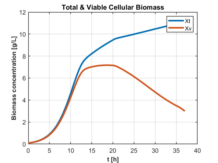
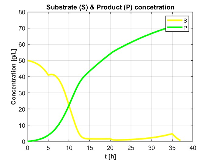
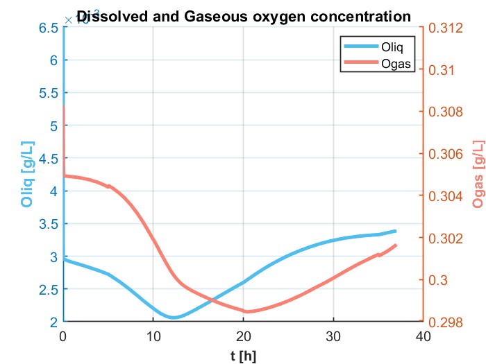
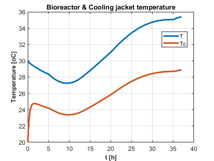
我正在尝试模拟一个DAE系统，它解决了用GEKKO生产乙醇的进料批量生物反应器的问题。这是为了以后我可以更容易地优化它，以最大限度地生产乙醇。它以前是在MATLAB中解决的，得到了如下数字所示的结果：

，

，

，

，

我现在的问题是，我不能用GEKKO产生相同的结果，给出所有相同的常量和变量的值。无法找到解决方案，但收敛的时间较短，例如: m.time= np.linspace(0、1、11)。知道我的代码出了什么问题吗？

需要解决的最初制度是：

from gekko import GEKKO
import numpy as np
import matplotlib.pyplot as plt


m = GEKKO(remote=False)
# Create time vector: t=[0, 0.1, 0.2,...,36.9,37], [hours]
nt = 371
m.time = np.linspace(0,37,nt)

# Define constants and parameters
#################################
# Kinetic Parameters
a1     = m.Const(value=0.05, name='a1')     # Ratkowsky parameter [oC-1 h-0.5]
aP     = m.Const(value=4.50, name='aP')     # Growth-associated parameter for EtOh production [-]
AP1    = m.Const(value=6.0, name='AP1')     # Activation energy parameter for EtOh production [oC]
AP2    = m.Const(value=20.3, name='AP2')    # Activation energy parameter for EtOh production [oC]
b1     = m.Const(value=0.035, name='b1')    # Parameter in the exponential expression of the maximum specific growth rate expression [oC-1]
b2     = m.Const(value=0.15, name='b2')     # Parameter in the exponential expression of the maximum specific growth rate expression [oC-1]
b3     = m.Const(value=0.40, name='b3')     # Parameter in the exponential expression of the specific death rate expression [oC-1]
c1     = m.Const(value=0.38, name='c1')     # Constant decoupling factor for EtOh [gP gX-1 h-1]
c2     = m.Const(value=0.29, name='c2')     # Constant decoupling factor for EtOh [gP gX-1 h-1]
k1     = m.Const(value=3, name='k1')        # Parameter in the maximum specific growth rate expression [oC]
k2     = m.Const(value=55, name='k2')       # Parameter in the maximum specific growth rate expression [oC]
k3     = m.Const(value=60, name='k3')       # Parameter in the growth-inhibitory EtOH concentration expression [oC]
k4     = m.Const(value=50, name='k4')       # Temperature at the inflection point of the specific death rate sigmoid curve [oC]
Pmaxb  = m.Const(value=90, name='Pmaxb')    # Temperature-independent product inhibition constant [g L-1]
PmaxT  = m.Const(value=90, name='PmaxT')    # Maximum value of product inhibition constant due to temperature [g L-1]
Kdb    = m.Const(value=0.025, name='Kdb')   # Basal specific cellular biomass death rate [h-1]
KdT    = m.Const(value=30, name='KdT')      # Maximum value of specific cellular biomass death rate due to temperature [h-1]
KSX    = m.Const(value=5, name='KSX')       # Glucose saturation constant for the specific growth rate [g L-1]
KOX    = m.Const(value=0.0005, name='KOX')  # Oxygen saturation constant for the specific growth rate [g L-1]
qOmax  = m.Const(value=0.05, name='qOmax')  # Maximum specific oxygen consumption rate [h-1]

# Metabolic Parameters
YPS    = m.Const(value=0.51, name='YPS')    # Theoretical yield of EtOH on glucose [gP gS-1]
YXO    = m.Const(value=0.97, name='YXO')    # Theoretical yield of biomass on oxygen [gX gO-1]
YXS    = m.Const(value=0.53, name='YXS')    # Theoretical yield of biomass on glucose [gX gS-1]

# Physicochemical and thermodynamic parameters
Chbr   = m.Const(value=4.18, name='Chbr')      # Heat capacity of the mass of reaction [J g-1 oC-1]
Chc    = m.Const(value=4.18, name='Chc')       # Heat capacity of cooling agent [J g-1 oC-1]
deltaH = m.Const(value=518.e3, name='deltaH')  # Heat of reaction of fermentation [J mol-1 O2]
Tref   = m.Const(value=25, name='Tref')        # Reference temperature [oC]
KH     = m.Const(value=200, name='KH')         # Henry's constant for oxygen in the fermentation broth [atm L mol-1]
z      = m.Const(value=0.792, name='z')        # Oxygen compressibility factor [-]
R      = m.Const(value=0.082, name='R')        # Ideal gas constant [L atm mol-1 oC-1]
kla0   = m.Const(value=100, name='kla0')       # Temperature-independent volumetric oxygen transfer coefficient [-h]
KT     = m.Const(value=36.e4, name='KT')       # Heat transfer coefficient [J h-1 m-2 oC-1]
rho    = m.Const(value=1080, name='rho')       # Density of the fermentation broth [g L-1]
rhoc   = m.Const(value=1000, name='rhoc')      # Density of the cooling agent [g L-1]
MO     = m.Const(value=15.999, name='MO')      # Molecular weight of oxygen [g mol-1]

# Bioreactor design data
AT     = m.Const(value=1, name='AT')          # Bioreactor heat transfer area [m2]
V      = m.Const(value=2000, name='V')        # Bioreactor working volume [L]
Vcj    = m.Const(value=250, name='Vcj')       # Cooling jacket volume [L]
Ogasin = m.Const(value=0.305, name='Ogasin')  # Oxygen concentration in airflow inlet [g L-1]

# Define variables
##################
mi = m.Var(name='mi')
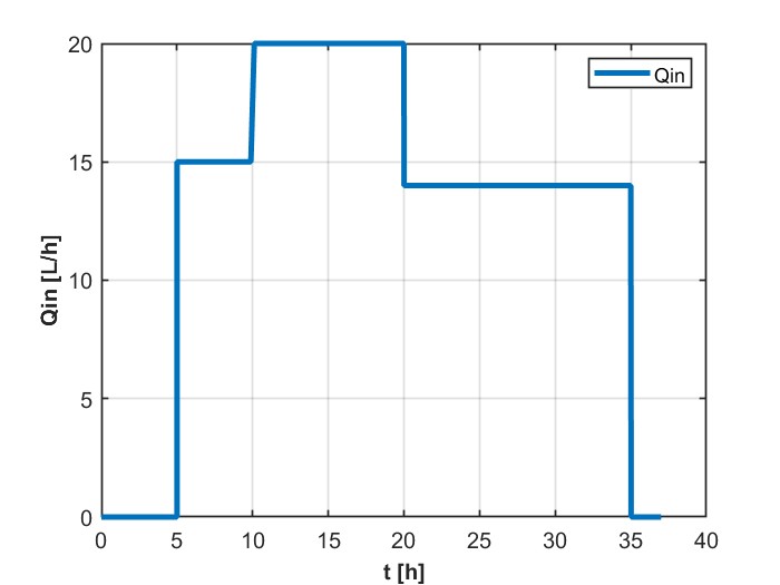
# I want Qin to be a step function: Qin = Qin0 + 15H(t-5) + 5H(t-10) - 6H(t-20) - 14H(t-35), where H(t-t0) heaviside function
Qin_step = np.zeros(nt)
Qin_step[50:101]  = 15
Qin_step[101:201] = 20
Qin_step[201:350] = 14
Qin  = m.Param(value=Qin_step, name='Qin')
# Fixed variables, they are constant throughout the time horizon
Xtin = m.FV(value=0, name='Xtin')
Xvin = m.FV(value=0, name='Xvin')
Qe   = m.FV(value=0, name='Qe')
Sin  = m.FV(value=400, lb=0, ub=1500)
Pin  = m.FV(value=0, name='Pin')
Fc   = m.FV(value=40, name='Fc')
Fair = m.FV(value=60000, name='Fair')
Tin  = m.FV(value=30, name='Tin')
Tcin = m.FV(value=15, name='Tcin')

Vl     = m.Var(value=1000, lb=-0.0, ub=0.75*V, name='Vl')
Xt     = m.Var(value=0.1, lb=-0.0, ub=10, name='Xt')
Xv     = m.Var(value=0.1, lb=-0.0, ub=10, name='Xv')
S      = m.Var(value=400, lb=+0.0, ub=10000, name='S')
P      = m.Var(value=0, name='P')
Ol     = m.Var(value=0.0065, name= 'Ol')
Og     = m.Var(value=0.305, name='Og')
T      = m.Var(value=30, lb=20, ub=40, name='T')
Tc     = m.Var(value=20, lb=0, ub=30, name='Tc')
Sf_cum = m.Var(value=0, name='Sf_cum')
t      = m.Var(value=0, name='Time')

# Define algebraic equations
############################
# Specific growth rate of cell mass
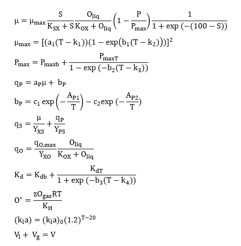
mimax = m.Intermediate(((a1*(T - k1))*(1 - m.exp(b1 * (T - k2)) )) ** 2)
Pmax = m.Intermediate(Pmaxb + PmaxT/(1- m.exp(-b2*(T-k3))))
m.Equation(mi == mimax * (S / (KSX + S)) * (Ol / (KOX + Ol)) * (1 - P / Pmax) * (1 / (1 + m.exp(-(100 - S)))))
mi = m.if3(condition=mi, x1=0, x2=mi)
# Specific production rate of EtOH
bP = m.if3(condition=S, x1=0, x2=c1*m.exp(-AP1/T) - c2*m.exp(-AP2/T))
qP = m.Intermediate(aP*mi + bP)
# Specific consumption rate of glucose
qS = m.Intermediate(mi/YXS + qP/YPS)
# Specific consumption rate of oxygen
qO = m.Intermediate(qOmax*Ol/YXO/(KOX+Ol))
# Specific biological deactivation rate of cell mass
Kd = m.Intermediate(Kdb + KdT/(1+m.exp(-b3*(T-k4))))
# Saturation concentration of oxygen in culture media
Ostar = m.Intermediate(z*Og*R*T/KH)
# Oxygen mass transfer coefficient
kla = m.Intermediate(kla0*1.2**(T-20))
# Bioreactor phases equation
Vg = m.Intermediate(V - Vl)

# Define differential equations
###############################
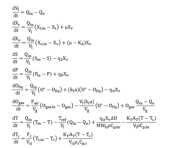
m.Equation(Vl.dt()     == Qin - Qe)
m.Equation(Xt.dt()     == Qin/Vl*(Xtin-Xt) + mi*Xv)
m.Equation(Xv.dt()     == Qin/Vl*(Xvin-Xv) + Xv*(mi-Kd))
m.Equation(S.dt()      == Qin/Vl*(Sin-S) - qS*Xv)
m.Equation(P.dt()      == Qin/Vl*(Pin - P) + qP*Xv)
m.Equation(Ol.dt()     == Qin/Vl*(Ostar-Ol) + kla*(Ostar-Ol) - qO*Xv)
m.Equation(Og.dt()     == Fair/Vg*(Ogasin-Og) - Vl*kla/Vg*(Ostar-Ol) + Og*(Qin-Qe)/Vg)
m.Equation(T.dt()      == Qin/Vl*(Tin-T) - Tref/Vl*(Qin-Qe) + qO*Xv*deltaH/MO/rho/Chbr - KT*AT*(T-Tc)/Vl/rho/Chbr)
m.Equation(Tc.dt()     == Fc/Vcj*(Tcin - Tc) + KT*AT*(T-Tc)/Vcj/rhoc/Chc)
m.Equation(Sf_cum.dt() == Qin*Sin)
m.Equation(t.dt()      == 1)

# solve ODE
m.options.IMODE = 6
# m.open_folder()
m.solve(display=True)

# Plot results
plt.figure(1)
plt.title('Total & Viable Cellular Biomass')
plt.plot(m.time, Xv.value, label='Xv')
plt.plot(m.time, Xt.value, label='Xt')
plt.legend()
plt.ylabel('Biomass concentration [g/L]')
plt.xlabel('Time [h]')
plt.grid()
plt.minorticks_on()
plt.ylim(0)
plt.xlim(m.time[0],m.time[-1])
plt.tight_layout()

plt.figure(2)
plt.title('Substrate (S) & Product (P) concentration')
plt.plot(m.time, S.value, label='S')
plt.plot(m.time, P.value, label='P')
plt.legend()
plt.ylabel('Concentration [g/L]')
plt.xlabel('Time [h]')
plt.grid()
plt.minorticks_on()
plt.ylim(0)
plt.xlim(m.time[0],m.time[-1])
plt.tight_layout()

plt.figure(3)
plt.title('Bioreactor & Cooling jacket temperature')
plt.plot(m.time, T.value, label='T')
plt.plot(m.time, Tc.value, label='Tc')
plt.legend()
plt.ylabel('Temperature [oC]')
plt.xlabel('Time [h]')
plt.grid()
plt.minorticks_on()
plt.ylim(0)
plt.xlim(m.time[0],m.time[-1])
plt.tight_layout()

fig4, ax = plt.subplots()
ax.title.set_text('Dissolved & Gaseous Oxygen concentration')
lns1 = ax.plot(m.time, Ol.value, label='[Oliq]', color='c')
ax.set_xlabel('Time [h]')
ax.set_ylabel('Oliq [g/L]', color='c')
ax.minorticks_on()
ax2 = ax.twinx()
lns2 = ax2.plot(m.time, Og.value, label='[Ogas]', color='y')
ax2.set_ylabel('Ogas [g/L]', color='y')
ax2.minorticks_on()
lns = lns1 + lns2
labs = [l.get_label() for l in lns]
ax.legend(lns, labs, loc='best')
ax.grid()
fig4.tight_layout()
plt.figure(4)

plt.figure(5)
plt.title('Feeding Policy')
plt.plot(m.time, Qin.value, label='Qin')
plt.legend()
plt.ylabel('Qin [L/h]')
plt.xlabel('Time [h]')
plt.grid()
plt.minorticks_on()
plt.ylim(0)
plt.xlim(m.time[0],m.time[-1])
plt.tight_layout()

plt.show()

python

simulation

gekko

回答 1

Stack Overflow用户

回答已采纳

发布于 2022-11-09 02:51:40

很好的申请！以下是一些改进收敛性的建议。

在模拟时移除上下界。这导致了“找不到解决方案”错误。

Vl     = m.Var(value=1000, name='Vl') # lb=-0.0, ub=0.75*V
Xt     = m.Var(value=0.1,  name='Xt') # lb=-0.0, ub=10
Xv     = m.Var(value=0.1,  name='Xv') # lb=-0.0, ub=10
S      = m.Var(value=400,  name='S')  # lb=+0.0, ub=10000
P      = m.Var(value=0, name='P')
Ol     = m.Var(value=0.0065, name= 'Ol')
Og     = m.Var(value=0.305, name='Og')
T      = m.Var(value=30, name='T')    # lb=20, ub=40
Tc     = m.Var(value=20, name='Tc')   # lb=0, ub=30

重新安排方程，以避免除以零(如有可能)。对于大多数方程，体积项可以移动到方程的左边，以避免分母中的变量。

m.Equation(Vl.dt()     == Qin - Qe)
m.Equation(Vl*Xt.dt()  == Qin*(Xtin-Xt) + mi*Vl*Xv)
m.Equation(Vl*Xv.dt()  == Qin*(Xvin-Xv) + Xv*Vl*(mi-Kd))
m.Equation(Vl*S.dt()   == Qin*(Sin-S) - qS*Vl*Xv)
m.Equation(Vl*P.dt()   == Qin*(Pin - P) + qP*Vl*Xv)
m.Equation(Vl*Ol.dt()  == Qin*(Ostar-Ol)   + Vl*kla*(Ostar-Ol) - qO*Vl*Xv)
m.Equation(Vg*Og.dt()  == Fair*(Ogasin-Og) - Vl*kla*(Ostar-Ol) + Og*(Qin-Qe))
m.Equation(Vl*T.dt()   == Qin*(Tin-T) - Tref*(Qin-Qe) \
                          + Vl*qO*Xv*deltaH/MO/rho/Chbr - KT*AT*(T-Tc)/rho/Chbr)
m.Equation(Vcj*Tc.dt() == Fc*(Tcin - Tc) + KT*AT*(T-Tc)/rhoc/Chc)
m.Equation(Sf_cum.dt() == Qin*Sin)

使用APOPT解算器提高速度，增加NODES=3以提高精度。IMODE=7是一种在零自由度情况下提高求解速度的顺序仿真(仿真，#equations=#variables)。

m.options.SOLVER= 1
m.options.IMODE = 7
m.options.NODES = 3

下面是一种基于时间的步骤输入的更简单的定义方法。

# I want Qin to be a step function:
#   Qin = Qin0 + 15H(t-5) + 5H(t-10) - 6H(t-20) - 14H(t-35)
#   where H(t-t0) heaviside function
Qin_step = np.zeros(nt)
Qin_step[np.where(tm>=5)]  += 15
Qin_step[np.where(tm>=10)] += 5
Qin_step[np.where(tm>=20)] -= 6
Qin_step[np.where(tm>=35)] -= 14
Qin  = m.Param(value=Qin_step, name='Qin')

避免if3() (如果可能)，并在变量定义中用下界替换：

#mi = m.if3(condition=mi, x1=0, x2=mi)
mi = m.Var(name='mi',lb=0)
m.Equation(mi == mimax * (S / (KSX+S)) * (Ol/(KOX + Ol)) \
                 * (1 - P/Pmax) * (1 / (1+m.exp(-(100-S)))))

或者松弛变量 slk，它避免了m.if3()引入的二进制交换变量。

slk  = m.Var(0,lb=0)
mi_u = m.Var(name='mi_u')
mi   = m.Var(name='mi',lb=0)
m.Equation(mi = mi_u + slk)
m.Minimize(slk)

(可选)如果出现收敛问题，则在开始时插入一些额外的小步骤。这在以后开始优化时非常有用。

# Create time vector: t=[0, 0.1, 0.2,...,36.9,37], [hours]
tm = np.linspace(0,37,371)
# Insert smaller time steps at the beginning
tm = np.insert(tm,1,[0.001,0.005,0.01,0.05])

(稍后)当您需要优化时，当您需要对优化问题进行初步猜测时，收敛到模拟中通常是很有帮助的。

m.options.IMODE=7
m.solve()
m.options.IMODE=6
m.solve()

这是完整的剧本。

from gekko import GEKKO
import numpy as np
import matplotlib.pyplot as plt

m = GEKKO(remote=False)
# Create time vector: t=[0, 0.1, 0.2,...,36.9,37], [hours]
tm = np.linspace(0,37,371)
# Insert smaller time steps at the beginning
tm = np.insert(tm,1,[0.001,0.005,0.01,0.05])
m.time = tm
nt = len(tm)

# Define constants and parameters
#################################
# Kinetic Parameters
a1     = m.Const(value=0.05, name='a1')     # Ratkowsky parameter [oC-1 h-0.5]
aP     = m.Const(value=4.50, name='aP')     # Growth-associated parameter for EtOh production [-]
AP1    = m.Const(value=6.0, name='AP1')     # Activation energy parameter for EtOh production [oC]
AP2    = m.Const(value=20.3, name='AP2')    # Activation energy parameter for EtOh production [oC]
b1     = m.Const(value=0.035, name='b1')    # Parameter in the exponential expression of the maximum specific growth rate expression [oC-1]
b2     = m.Const(value=0.15, name='b2')     # Parameter in the exponential expression of the maximum specific growth rate expression [oC-1]
b3     = m.Const(value=0.40, name='b3')     # Parameter in the exponential expression of the specific death rate expression [oC-1]
c1     = m.Const(value=0.38, name='c1')     # Constant decoupling factor for EtOh [gP gX-1 h-1]
c2     = m.Const(value=0.29, name='c2')     # Constant decoupling factor for EtOh [gP gX-1 h-1]
k1     = m.Const(value=3, name='k1')        # Parameter in the maximum specific growth rate expression [oC]
k2     = m.Const(value=55, name='k2')       # Parameter in the maximum specific growth rate expression [oC]
k3     = m.Const(value=60, name='k3')       # Parameter in the growth-inhibitory EtOH concentration expression [oC]
k4     = m.Const(value=50, name='k4')       # Temperature at the inflection point of the specific death rate sigmoid curve [oC]
Pmaxb  = m.Const(value=90, name='Pmaxb')    # Temperature-independent product inhibition constant [g L-1]
PmaxT  = m.Const(value=90, name='PmaxT')    # Maximum value of product inhibition constant due to temperature [g L-1]
Kdb    = m.Const(value=0.025, name='Kdb')   # Basal specific cellular biomass death rate [h-1]
KdT    = m.Const(value=30, name='KdT')      # Maximum value of specific cellular biomass death rate due to temperature [h-1]
KSX    = m.Const(value=5, name='KSX')       # Glucose saturation constant for the specific growth rate [g L-1]
KOX    = m.Const(value=0.0005, name='KOX')  # Oxygen saturation constant for the specific growth rate [g L-1]
qOmax  = m.Const(value=0.05, name='qOmax')  # Maximum specific oxygen consumption rate [h-1]

# Metabolic Parameters
YPS    = m.Const(value=0.51, name='YPS')    # Theoretical yield of EtOH on glucose [gP gS-1]
YXO    = m.Const(value=0.97, name='YXO')    # Theoretical yield of biomass on oxygen [gX gO-1]
YXS    = m.Const(value=0.53, name='YXS')    # Theoretical yield of biomass on glucose [gX gS-1]

# Physicochemical and thermodynamic parameters
Chbr   = m.Const(value=4.18, name='Chbr')      # Heat capacity of the mass of reaction [J g-1 oC-1]
Chc    = m.Const(value=4.18, name='Chc')       # Heat capacity of cooling agent [J g-1 oC-1]
deltaH = m.Const(value=518000, name='deltaH')  # Heat of reaction of fermentation [J mol-1 O2]
Tref   = m.Const(value=20, name='Tref')        # Reference temperature [oC]
KH     = m.Const(value=200, name='KH')         # Henry's constant for oxygen in the fermentation broth [atm L mol-1]
z      = m.Const(value=0.792, name='z')        # Oxygen compressibility factor [-]
R      = m.Const(value=0.082, name='R')        # Ideal gas constant [L atm mol-1 oC-1]
kla0   = m.Const(value=100, name='kla0')       # Temperature-independent volumetric oxygen transfer coefficient [-h]
KT     = m.Const(value=360000, name='KT')      # Heat transfer coefficient [J h-1 m-2 oC-1]
rho    = m.Const(value=1080, name='rho')       # Density of the fermentation broth [g L-1]
rhoc   = m.Const(value=1000, name='rhoc')      # Density of the cooling agent [g L-1]
MO     = m.Const(value=32.0, name='MO')        # Molecular weight of oxygen [g mol-1]

# Bioreactor design data
AT     = m.Const(value=1, name='AT')          # Bioreactor heat transfer area [m2]
V      = m.Const(value=1800, name='V')        # Bioreactor working volume [L]
Vcj    = m.Const(value=50, name='Vcj')       # Cooling jacket volume [L]
Ogasin = m.Const(value=0.305, name='Ogasin')  # Oxygen concentration in airflow inlet [g L-1]

# Define variables
##################
mi = m.Var(name='mi',lb=0)
# I want Qin to be a step function:
#   Qin = Qin0 + 15H(t-5) + 5H(t-10) - 6H(t-20) - 14H(t-35)
#   where H(t-t0) heaviside function
Qin_step = np.zeros(nt)
Qin_step[np.where(tm>=5)]  += 15
Qin_step[np.where(tm>=10)] += 5
Qin_step[np.where(tm>=20)] -= 6
Qin_step[np.where(tm>=35)] -= 14
Qin  = m.Param(value=Qin_step, name='Qin')
# Fixed variables, they are constant throughout the time horizon
Xtin = m.FV(value=0, name='Xtin')
Xvin = m.FV(value=0, name='Xvin')
Qe   = m.FV(value=0, name='Qe')
Sin  = m.FV(value=400, lb=0, ub=1500)
Pin  = m.FV(value=0, name='Pin')
Fc   = m.FV(value=40, name='Fc')
Fair = m.FV(value=60000, name='Fair')
Tin  = m.FV(value=30, name='Tin')
Tcin = m.FV(value=15, name='Tcin')

Vl     = m.Var(value=1000, name='Vl') # lb=-0.0, ub=0.75*V
Xt     = m.Var(value=0.1,  name='Xt') # lb=-0.0, ub=10
Xv     = m.Var(value=0.1,  name='Xv') # lb=-0.0, ub=10
S      = m.Var(value=50,  name='S')   # lb=+0.0, ub=10000
P      = m.Var(value=0, name='P')
Ol     = m.Var(value=0.0065, name= 'Ol')
Og     = m.Var(value=0.305, name='Og')
T      = m.Var(value=30, name='T')    # lb=20, ub=40
Tc     = m.Var(value=20, name='Tc')   # lb=0, ub=30
Sf_cum = m.Var(value=0, name='Sf_cum')
#t      = m.Var(value=0, name='Time')

# Define algebraic equations
############################
# Specific growth rate of cell mass
mimax = m.Intermediate(((a1*(T-k1))*(1-m.exp(b1*(T-k2))))** 2)
Pmax = m.Intermediate(Pmaxb + PmaxT/(1-m.exp(-b2*(T-k3))))
m.Equation(mi == mimax * (S / (KSX+S)) * (Ol/(KOX + Ol)) \
                 * (1 - P/Pmax) * (1 / (1+m.exp(-(100-S)))))
#mi = m.if3(condition=mi, x1=0, x2=mi)
# Specific production rate of EtOH
#bP = m.if3(condition=S, x1=0, x2=c1*m.exp(-AP1/T) - c2*m.exp(-AP2/T))
bP = m.Intermediate(c1*m.exp(-AP1/T) - c2*m.exp(-AP2/T))
qP = m.Intermediate(aP*mi + bP)
# Specific consumption rate of glucose
qS = m.Intermediate(mi/YXS + qP/YPS)
# Specific consumption rate of oxygen
qO = m.Intermediate(qOmax*Ol/YXO/(KOX+Ol))
# Specific biological deactivation rate of cell mass
Kd = m.Intermediate(Kdb + KdT/(1+m.exp(-b3*(T-k4))))
# Saturation concentration of oxygen in culture media
Ostar = m.Intermediate(z*Og*R*T/KH)
# Oxygen mass transfer coefficient
kla = m.Intermediate(kla0*1.2**(T-20))
# Bioreactor phases equation
Vg = m.Intermediate(V - Vl)

# Define differential equations
###############################
m.Equation(Vl.dt()     == Qin - Qe)
m.Equation(Vl*Xt.dt()  == Qin*(Xtin-Xt) + mi*Vl*Xv)
m.Equation(Vl*Xv.dt()  == Qin*(Xvin-Xv) + Xv*Vl*(mi-Kd))
m.Equation(Vl*S.dt()   == Qin*(Sin-S) - qS*Vl*Xv)
m.Equation(Vl*P.dt()   == Qin*(Pin - P) + qP*Vl*Xv)
m.Equation(Vl*Ol.dt()  == Qin*(Ostar-Ol)   + Vl*kla*(Ostar-Ol) - qO*Vl*Xv)
m.Equation(Vg*Og.dt()  == Fair*(Ogasin-Og) - Vl*kla*(Ostar-Ol) + Og*(Qin-Qe))
m.Equation(Vl*T.dt()   == Qin*(Tin-T) - Tref*(Qin-Qe) \
                          + Vl*qO*Xv*deltaH/MO/rho/Chbr - KT*AT*(T-Tc)/rho/Chbr)
m.Equation(Vcj*Tc.dt() == Fc*(Tcin - Tc) + KT*AT*(T-Tc)/rhoc/Chc)
m.Equation(Sf_cum.dt() == Qin*Sin)
#m.Equation(t.dt()      == 1)

# solve ODE
m.options.SOLVER= 1
m.options.IMODE = 7
m.options.NODES = 3
# m.open_folder()
m.solve(disp=False)

# Plot results
plt.figure(1)
plt.title('Total & Viable Cellular Biomass')
plt.plot(m.time, Xv.value, label='Xv')
plt.plot(m.time, Xt.value, label='Xt')
plt.legend()
plt.ylabel('Biomass concentration [g/L]')
plt.xlabel('Time [h]')
plt.grid()
plt.minorticks_on()
plt.ylim(0)
plt.xlim(m.time[0],m.time[-1])
plt.tight_layout()

plt.figure(2)
plt.title('Substrate (S) & Product (P) concentration')
plt.subplot(2,1,1)
plt.plot(m.time, S.value, label='S')
plt.legend(); plt.grid()
plt.ylabel('Conc [g/L]')
plt.subplot(2,1,2)
plt.plot(m.time, P.value, label='P')
plt.legend(); plt.grid()
plt.ylabel('Conc [g/L]')
plt.xlabel('Time [h]')
plt.minorticks_on()
plt.ylim(0)
plt.xlim(m.time[0],m.time[-1])
plt.tight_layout()

plt.figure(3)
plt.title('Bioreactor & Cooling jacket temperature')
plt.plot(m.time, T.value, label='T')
plt.plot(m.time, Tc.value, label='Tc')
plt.legend()
plt.ylabel('Temperature [oC]')
plt.xlabel('Time [h]')
plt.grid()
plt.minorticks_on()
plt.ylim(0)
plt.xlim(m.time[0],m.time[-1])
plt.tight_layout()

fig4, ax = plt.subplots()
ax.title.set_text('Dissolved & Gaseous Oxygen concentration')
lns1 = ax.plot(m.time, Ol.value, label='[Oliq]', color='c')
ax.set_xlabel('Time [h]')
ax.set_ylabel('Oliq [g/L]', color='c')
ax.minorticks_on()
ax2 = ax.twinx()
lns2 = ax2.plot(m.time, Og.value, label='[Ogas]', color='y')
ax2.set_ylabel('Ogas [g/L]', color='y')
ax2.minorticks_on()
lns = lns1 + lns2
labs = [l.get_label() for l in lns]
ax.legend(lns, labs, loc='best')
ax.grid()
fig4.tight_layout()
plt.figure(4)

plt.figure(5)
plt.title('Feeding Policy')
plt.plot(m.time, Qin.value, label='Qin')
plt.legend()
plt.ylabel('Qin [L/h]')
plt.xlabel('Time [h]')
plt.grid()
plt.minorticks_on()
plt.ylim(0)
plt.xlim(m.time[0],m.time[-1])
plt.tight_layout()

plt.figure(6)
plt.title('Check >=0 Constraints')
plt.subplot(2,1,1)
plt.plot(tm,bP.value,label='bP')
plt.legend(); plt.grid()
plt.subplot(2,1,2)
plt.plot(tm,mi.value,label='mi')
plt.legend(); plt.grid()

plt.show()

这些图用更新的参数复制Matlab图(谢谢建议)。如果我们能帮助进一步的问题，请告诉我们。

Python版本

下面是一个等效的Python版本。如果仍然需要，我创建它是为了帮助进行等效性测试。

import numpy as np
from scipy.integrate import odeint
from scipy.interpolate import interp1d
import matplotlib.pyplot as plt

#Simulate fed-batch operation
# Specify the simulation time (hrs)
tspan = np.linspace(0,37,371); t=tspan
# Specify values of control variables [Qin0 Xtin Xvin Qe Sin Fc Fair Tin Tcin]
u0 = [0.0,0.0,0.0,0.0,0.0,400,40,60000,30,15]
# Specify initial conditions [Xt Xv S P Oliq Ogas T Tc Vl Gloss MP]
x0 = [0.1,0.1,50,0,0.0065,0.305,30,20,1000,0.0,0.0]
ux0 = tuple(u0 + x0)

#Qin = 15*heaviside(t-5) + 5*heaviside(t-10)
#      - 6*heaviside(t-20) - 14*heaviside(t-35)
Qin = np.zeros_like(tspan)
Qin[np.where(tspan>=5)]  += 15
Qin[np.where(tspan>=10)] += 5
Qin[np.where(tspan>=20)] -= 6
Qin[np.where(tspan>=35)] -= 14
QinInterp = interp1d(tspan,Qin,bounds_error=False)

def ethanol(x,t,Qin0,Qin,Xtin,Xvin,Qe,Sin,Fc,Fair,
            Tin,Tcin,Xt0,Xv0,S0,P0,Oliq0,Ogas0,T0,
            Tc0,Vl0,Sf_cum0,Time0):
    ##    #Initial Conditions
    ##    Xt0 = u[10]     # Initial total cellular biomass, [g L-1]
    ##    Xv0 = u[11]     # Initial viable cellular biomass, [g L-1]
    ##    S0 = u[12]      # Initial substrate/Glucose concentration, [g L-1]
    ##    P0 = u[13]      # Initial product/Ethanol concentration, [g L-1]
    ##    Oliq0 = u[14]   # Initial Dissolved oxygen concentration, [g L-1]
    ##    Ogas0 = u[15]   # Initial Gas phase oxygen (bubbles) in the fermentation broth, [g L-1]
    ##    T0 = u[16]      # Initial Temperature in the bioreactor, [oC]
    ##    Tc0 = u[17]     # Initial Temperature of the cooling agent in the jacket, [oC]
    ##    Vl0 = u[18]     # Initial Culture volume in the bioreactor, [L]
    ##    Sf_cum0 = u[19] # Initial Cumulative substrate/glucose fed to the bioreactor, [g]
    ##    Time0 = u[20]   # Initial batch time, [h]
    ##    
    ##    #Control variables
    ##    Qin0 = u[0]        # Volumetric inflow rate, [l/h-1]
    ##    Qin = u[1]         # Volumetric inflow rate, [l/h-1]
    ##    Xtin = u[2]        # Total biomass concentration in the bioreactor feed, [g L-1]
    ##    Xvin = u[3]        # Viable biomass concentration in the bioreactor feed, [g L-1]
    ##    Qe = u[4]          # Volumetric outflow rate, [l/h-1]
    ##    Sin = u[5]         # Substrate/Glucose concentration in bioreactor feed, [g L-1]
    ##    Fc = u[6]          # Cooling agent inlet volumetric flowrate, [L h-1]
    ##    Fair = u[7]        # Airflow inlet volumetric flowrate, [L h-1]
    ##    Tin = u[8]         # Temperature of bioreactor feed, [oC]
    ##    Tcin = u[9]        # Temperature of cooling agent inlet, [oC]

    # 1D Interpolation for Qin
    Qin = QinInterp(t)
    
    #Definition of model parameters
    #Kinetic parameters
    a1 = 0.05    # Ratkowsky parameter [oC-1 h-0.5]
    aP = 4.50    # Growth-associated parameter for ethanol production, [-]
    AP1 = 6.0    # Activation energy parameter for ethanol production, [oC]
    AP2 = 20.3   # Activation energy parameter for ethanol production, [oC]
    b1 = 0.035   # Parameter in the exponential expression of the maximum specific growth rate np.expression, [oC-1]
    b2 = 0.15    # Parameter in the exponential expression of the growth inhibitory ethanol concentration np.expression, [oC-1]
    b3 = 0.40    # Parameter in the exponential np.expression of the specific death rate expression,[oC-1]
    c1 = 0.38    # Constant decoupling factor for ethanol production, [gP gX-1 h-1]
    c2 = 0.29    # Constant decoupling factor for ethanol production, [gP gX-1 h-1]
    k1 = 3.00    # Parameter in the maximum specific growth rate expression, [oC]
    k2 = 55.0    # Parameter in the maximum specific growth rate expression, [oC]
    k3 = 60.0    # Parameter in the growth-inhibitory ethanol concentration expression, [oC]
    k4 = 50.0    # Temperature at the inflection point of the specific death rate sigmoid curve, [oC]
    Pmaxb = 90   # Temperature-independent product inhibition constant, [g L-1]
    PmaxT = 90   # Maximum value of product inhibition constant due to temperature, [g L-1]
    Kdb = 0.025  # Basal specific cellular biomass death rate, [h-1]
    KdT = 30.00  # Maximum value of specific cellular biomass death rate due to temperature, [h-1]
    KSX = 5      # Glucose saturation constant for the specific growth rate, [g L-1]
    KOX = 0.0005 # Oxygen saturation constant for the specific growth rate, [g L-1]
    qOmax = 0.05 # Maximum specific oxygen consumption rate, [h-1]
    
    #Metabolic parameters
    YPS = 0.51 # Theoretical yield of ethanol on glucose, [gP gS-1]
    YXO = 0.97 # Theoretical yield of biomass on oxygen, [gX gO-1]
    YXS = 0.53 # Theoretical yield of biomass on glucose, [gX gS-1]
    
    #Physicochemical and thermodynamic parameters
    Chbr = 4.18     # Heat capacity of the mass of reaction, [J g-1 oC-1]
    Chc = 4.18      # Heat capacity of the cooling agent, [J g-1 oC-1]
    DeltaH = 518000 # Heat of reaction of fermentation, [J mol-1 O2]
    Tref = 20       # Reference temperature, [oC]
    KH = 200        # Henry's constant for oxygen in the fermentation broth, [atm L mol-1]
    z = 0.792       # Oxygen compressibility factor, [-]
    R = 0.082       # Ideas gas constant, [L atm mol-1 oC-1]
    kla0 = 100      # Temperature-independent volumetric oxygen transfer coefficient, [h-1]
    KT = 360000     # Heat transfer coefficient, [J h-1 m-2 ??C-1]
    rho = 1080      # Density of the fermentation broth, [g L-1]
    rhoc = 1000     # Density of the cooling agent, [g L-1]
    MO = 32.0       # Molecular weight of oxygen (O2), [g mol-1]
    
    #Bioreactor design data
    AT = 1.0       # Bioreactor heat transfer area, [m2]
    V = 1800       # Bioreactor working volume, [L]
    Vcj = 50       # Cooling jacket volume, [L]
    Ogasin = 0.305 # Oxygen concentration in airflow inlet, [g L-1]
    
    #Definition of model variables
    #State variables
    Xt = x[0]      # Total cellular biomass, [g L-1]
    Xv = x[1]      # Viable cellular biomass, [g L-1]
    S = x[2]       # Substrate/Glucose concentration, [g L-1]
    P = x[3]       # Product/Ethanol concentration, [g L-1]
    Oliq = x[4]    # Dissolved oxygen concentration, [g L-1]
    Ogas = x[5]    # Gas phase oxygen (bubbles) in the fermentation broth, [g L-1]
    T = x[6]       # Temperature in the bioreactor, [oC]
    Tc = x[7]      # Temperature of the cooling agent in the jacket, [oC]
    Vl = x[8]      # Culture volume in the bioreactor, [L]
    Sf_cum = x[9]  # Cumulative amount of substrate/glucose fed to the bioreactor, [g]
    Time = x[10]   # Batch time, [h]
        
    # Definition of model equations
    # Kinetic rates
    # -----------------------------
    # Specific growth rate, [h-1] 
    mmax = ((a1*(T-k1))*(1-np.exp(b1*(T-k2))))**2
    Pmax = Pmaxb + PmaxT/(1-np.exp(-b2*(T-k3)))
    m1 = mmax * S/(KSX + S) * Oliq/(KOX + Oliq) * (1 - P/Pmax) * 1/(1+np.exp(-(100-S)/1)) # Specific growth rate, [h-1] 
    if m1 >= 0:
        m = m1
    else:
        m=0.0
    # Non-growth-associated ethanol specific production rate, [h-1]
    if S > 0:
        bP = c1 * np.exp(-AP1/T) - c2 * np.exp(-AP2/T)  # Non-growth-associated ethanol specific production rate, [h-1]
    else:
        bP = 0.0
    qP = aP*m + bP
    # Ethanol consumption specific rate
    qS = m/YXS + qP/YPS
    # Oxygen consumption specific rate
    qO = qOmax*Oliq/YXO/(KOX + Oliq)
    # Specific biological deactivation rate of cell mass
    Kd = Kdb + KdT/(1+np.exp(-b3*(T-k4)))
    # Saturation concentration of oxygen in culture media
    Osat = z*Ogas*R*T/KH
    # Oxygen mass transfer coefficient
    kla = kla0*1.2**(T-20)
    # Volume of the gas phase in the bioreactor
    Vg = V - Vl
        
    #Material balances
    #-----------------
    # Volume of liquid culture
    dVl = Qin - Qe
    # Total cell mass
    dXt = m*Xv + Qin/Vl*(Xtin-Xt)
    # Total mass of biologically active cells
    dXv = (m-Kd)*Xv + Qin/Vl*(Xvin-Xv)
    # Glucose concentration
    dS = Qin/Vl*(Sin-S) - qS*Xv
    # Ethanol concentration
    dP = Qin/Vl*(-P) + qP*Xv
    # Disolved oxygen
    dOliq = Qin/Vl*(Osat - Oliq) + kla*(Osat-Oliq) - qO*Xv
    # Oxygen gas phase
    dOgas = Fair/Vg*(Ogasin-Ogas) - Vl*kla/Vg*(Osat - Oliq) + Ogas*(Qin-Qe)/Vg
    
    # Energy balances
    #---------------
    # Bioreactor temprature
    dT = Qin/Vl*(Tin-T) - Tref/Vl*(Qin-Qe) + qO*Xv*DeltaH/MO/rho/Chbr - KT*AT*(T-Tc)/Vl/rho/Chbr
    # Cooling agent temperature
    dTc = Fc/Vcj*(Tcin-Tc) + KT*AT*(T-Tc)/Vcj/rhoc/Chc
    
    # Yields & Productivity
    #---------------------
    # Cumulative amount of glucose fed to the bioreactor
    dSf_cum = Sin*Qin
    dTime = 1
    
    # Definition of state derivatives vector
    # State derivatives
    dxdt = [dXt,dXv,dS,dP,dOliq,dOgas,dT,dTc,dVl,dSf_cum,dTime]
    
    # [dxdt,mmax,Pmax,bP,m,Kd,Qin]
    return dxdt

# test function
print(ethanol(x0,0.0,*ux0))

# Simulate the bioreactor operation until the selected time tf
x = odeint(ethanol,x0,tspan,args=ux0)

#plots Results
#Total and Viable Cellular Biomass
plt.figure()
plt.plot(tspan,x[:,0])
plt.plot(tspan,x[:,1])
plt.title('Total & Viable Cellular Biomass')
plt.ylabel('Biomass concentration [g/L]') 
plt.xlabel('t [h]')
plt.legend(['Xt','Xv'])

plt.figure()
plt.title('Substrate (S) & Product (P) concentration')
plt.plot(tspan,x[:,2], label='S')
plt.plot(tspan,x[:,3], label='P')
plt.legend(); plt.grid()
plt.ylabel('Conc [g/L]')
plt.xlabel('Time [h]')
plt.minorticks_on()
plt.ylim(0)
plt.xlim(t[0],t[-1])
plt.tight_layout()

plt.figure()
plt.title('Bioreactor & Cooling jacket temperature')
plt.plot(tspan,x[:,6], label='T')
plt.plot(tspan,x[:,7], label='Tc')
plt.legend()
plt.ylabel('Temperature [oC]')
plt.xlabel('Time [h]')
plt.grid()
plt.minorticks_on()
plt.ylim(0)
plt.xlim(t[0],t[-1])
plt.tight_layout()

fig4, ax = plt.subplots()
ax.title.set_text('Dissolved & Gaseous Oxygen concentration')
lns1 = ax.plot(t,x[:,4], label='[Oliq]', color='c')
ax.set_xlabel('Time [h]')
ax.set_ylabel('Oliq [g/L]', color='c')
ax.minorticks_on()
ax2 = ax.twinx()
lns2 = ax2.plot(t,x[:,5], label='[Ogas]', color='y')
ax2.set_ylabel('Ogas [g/L]', color='y')
ax2.minorticks_on()
lns = lns1 + lns2
labs = [l.get_label() for l in lns]
ax.legend(lns, labs, loc='best')
ax.grid()
fig4.tight_layout()

plt.figure()
plt.title('Feeding Policy')
plt.plot(tspan, Qin, label='Qin')
plt.legend()
plt.ylabel('Qin [L/h]')
plt.xlabel('Time [h]')
plt.grid()
plt.minorticks_on()
plt.ylim(0)
plt.xlim(tspan[0],tspan[-1])
plt.tight_layout()

plt.show()

票数 3

页面原文内容由Stack Overflow提供。腾讯云小微IT领域专用引擎提供翻译支持

原文链接：

https://stackoverflow.com/questions/74362585

复制

相似问题

问利用GEKKO生物反应器模拟乙醇生产
EN

回答 1

Stack Overflow用户

社区

活动

圈层

关于

腾讯云开发者

热门产品

热门推荐

更多推荐

问利用GEKKO生物反应器模拟乙醇生产EN

回答 1

Stack Overflow用户

社区

活动

圈层

关于

腾讯云开发者

热门产品

热门推荐

更多推荐

问利用GEKKO生物反应器模拟乙醇生产
EN