动力系统分岔图

Question

TL：博士

如何在Python中实现季节性强制流行病学模型的分叉图，例如SEIR (易感、暴露、感染、恢复)？我已经知道如何实现模型本身并显示抽样时间序列(参见这个堆叠溢出问题)，但我很难从教科书中复制分叉图。

上下文与我的尝试

我试图复制“人类和动物传染病建模”(Keeling，2007)一书中的数字，以验证我对模型的实现，并学习/可视化不同的模型参数如何影响动力系统的演化。以下是教科书上的数字。

​

​

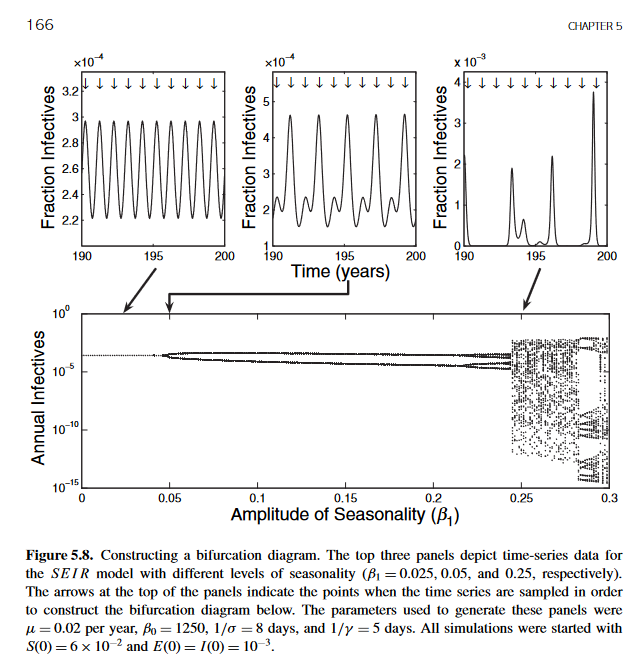
我已经为使用逻辑映射的例子找到了分支图的实现(请参阅这个ipython食谱 - 肾盂分叉，和这个堆栈过流问题)。我从这些实现中得到的主要结论是，分岔图上的一个点具有一个x分量，它的x分量等于可变参数的某个特定值(例如，Beta 1= 0.025)，并且它的y分量是给定模型/函数在时间t处的解(数值或其他)。在这个问题的末尾，我使用这个逻辑实现代码部分中的plot_bifurcation函数。

​

​

​

​

问题

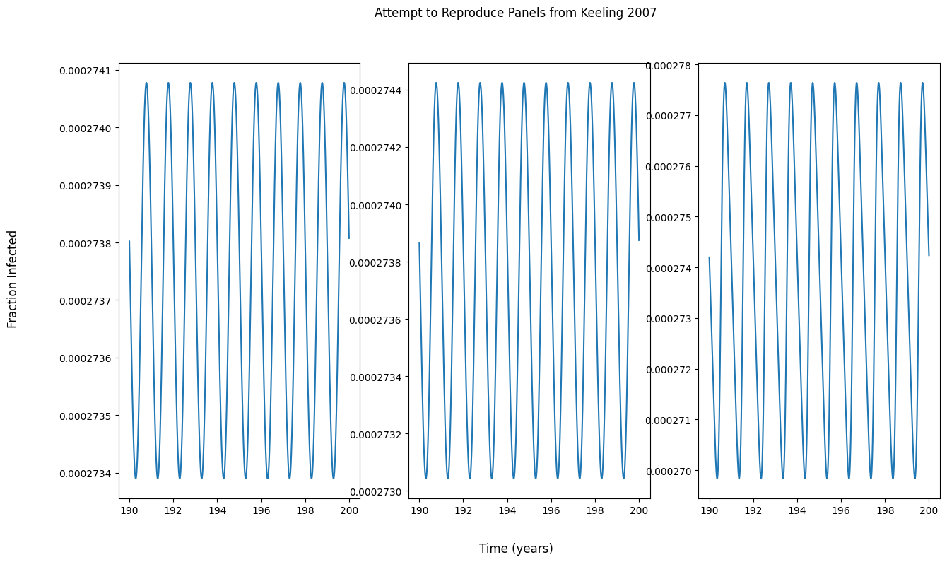
为什么我的面板输出与图中的不匹配？我假设，如果没有面板匹配教科书中的输出，我就无法从教科书中复制分叉图。

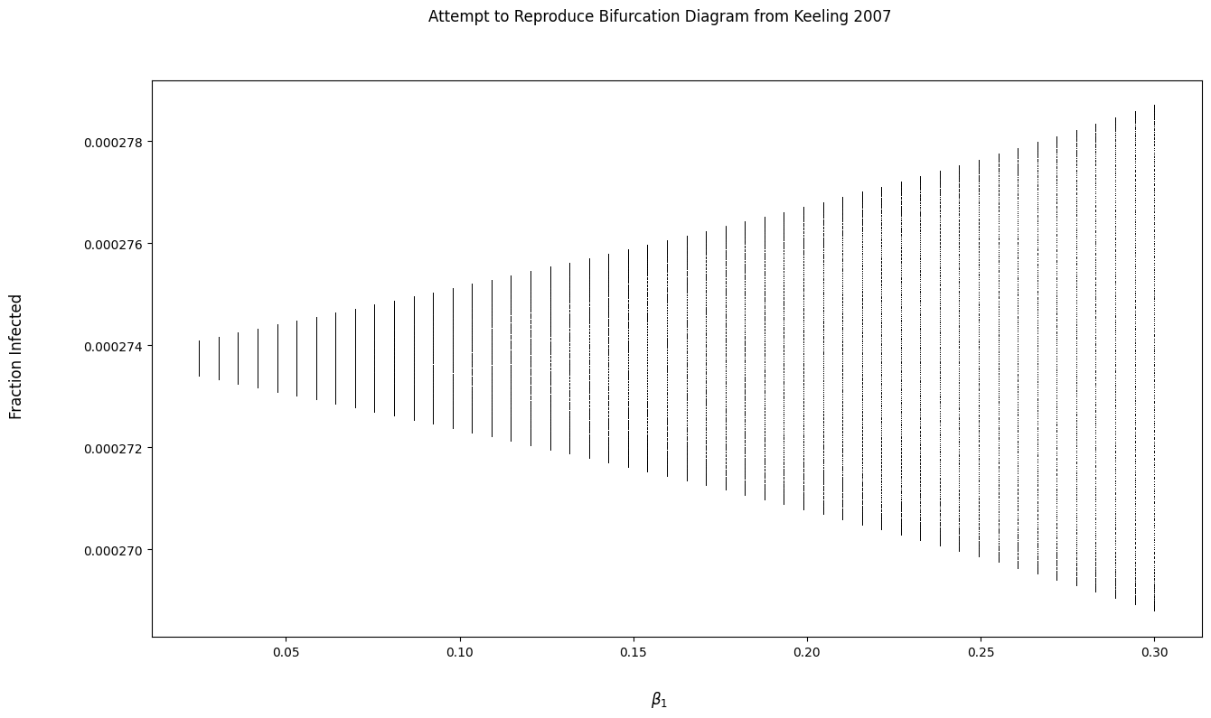
我试图实现一个函数来生成分岔图，但是输出看起来真的很奇怪。我对分叉图有什么误解吗？

注意:在代码执行期间，我没有收到警告/错误。

代码复制我的数字

from typing import Callable, Dict, List, Optional, Any
import numpy as np
import matplotlib.pyplot as plt
from scipy.integrate import odeint

def seasonal_seir(y: List, t: List, params: Dict[str, Any]):
    """Seasonally forced SEIR model.
    
    Function parameters much match with those required
    by `scipy.integrate.odeint`

    Args:
        y: Initial conditions.
        t: Timesteps over which numerical solution will be computed.
        params: Dict with the following key-value pairs:
            beta_zero -- Average transmission rate.
            beta_one  -- Amplitude of seasonal forcing.
            omega     -- Period of forcing.
            mu        -- Natural mortality rate.
            sigma     -- Latent period for infection.
            gamma     -- Recovery from infection term.

    Returns:
        Tuple whose components are the derivatives of the
        susceptible, exposed, and infected state variables
        w.r.t to time.

    References:
        [SEIR Python Program from Textbook](http://homepages.warwick.ac.uk/~masfz/ModelingInfectiousDiseases/Chapter2/Program_2.6/Program_2_6.py)
        [Seasonally Forced SIR Program from Textbook](http://homepages.warwick.ac.uk/~masfz/ModelingInfectiousDiseases/Chapter5/Program_5.1/Program_5_1.py)
    """
    beta_zero = params['beta_zero']
    beta_one = params['beta_one']
    omega = params['omega']
    mu = params['mu']
    sigma = params['sigma']
    gamma = params['gamma']

    s, e, i = y 
    beta = beta_zero*(1 + beta_one*np.cos(omega*t))
    sdot = mu - (beta * i + mu)*s
    edot = beta*s*i - (mu + sigma)*e
    idot = sigma*e - (mu + gamma)*i
    return sdot, edot, idot

def plot_panels(
    model: Callable,
    model_params: Dict, 
    panel_param_space: List, 
    panel_param_name: str,
    initial_conditions: List,
    timesteps: List,
    odeint_kwargs: Optional[Dict] = dict(),
    x_ticks: Optional[List] = None,
    time_slice: Optional[slice] = None,
    state_var_ix: Optional[int] = None,
    log_scale: bool = False):
    """Plot panels that are samples of the parameter space for bifurcation.

    Args:
        model: Function that models dynamical system. Returns dydt.
        model_params: Dict whose key-value pairs are the names
            of parameters in a given model and the values of those parameters.
        bifurcation_parameter_space: List of varied bifurcation parameters.
        bifuraction_parameter_name: The name o the bifurcation parameter.
        initial_conditions: Initial conditions for numerical integration.
        timesteps: Timesteps for numerical integration.
        odeint_kwargs: Key word args for numerical integration.
        state_var_ix: State variable in solutions to use for plot.
        time_slice: Restrict the bifurcation plot to a subset
            of the all solutions for numerical integration timestep space.
    
    Returns:
        Figure and axes tuple.
    """

    # Set default ticks
    if x_ticks is None:
        x_ticks = timesteps

    # Create figure
    fig, axs = plt.subplots(ncols=len(panel_param_space))

    # For each parameter that is varied for a given panel
    # compute numerical solutions and plot
    for ix, panel_param in enumerate(panel_param_space):

        # update model parameters with the varied parameter
        model_params[panel_param_name] = panel_param

        # Compute solutions
        solutions = odeint(
            model,
            initial_conditions,
            timesteps,
            args=(model_params,),
            **odeint_kwargs)

        # If there is a particular solution of interst, index it
        # otherwise squeeze last dimension so that [T, 1] --> [T]
        # where T is the max number of timesteps
        if state_var_ix is not None:
            solutions = solutions[:, state_var_ix]

        elif state_var_ix is None and solutions.shape[-1] == 1:
            solutions = np.squeeze(solutions)
        
        else:
            raise ValueError(
                f'solutions to model are rank-2 tensor of shape {solutions.shape}'
                ' with the second dimension greater than 1. You must pass'
                ' a value to :param state_var_ix:')

        # Slice the solutions based on the desired time range
        if time_slice is not None:
            solutions = solutions[time_slice]

        # Natural log scale the results
        if log_scale:
            solutions = np.log(solutions)

        # Plot the results
        axs[ix].plot(x_ticks, solutions)

    return fig, axs

def plot_bifurcation(
    model: Callable,
    model_params: Dict,
    bifurcation_parameter_space: List,
    bifurcation_param_name: str,
    initial_conditions: List,
    timesteps: List,
    odeint_kwargs: Optional[Dict] = dict(),
    state_var_ix: Optional[int] = None,
    time_slice: Optional[slice] = None,
    log_scale: bool = False):
    """Plot a bifurcation diagram of state variable from dynamical system.

    Args:
        model: Function that models system. Returns dydt.
        model_params: Dict whose key-value pairs are the names
            of parameters in a given model and the values of those parameters.
        bifurcation_parameter_space: List of varied bifurcation parameters.
        bifuraction_parameter_name: The name o the bifurcation parameter.
        initial_conditions: Initial conditions for numerical integration.
        timesteps: Timesteps for numerical integration.
        odeint_kwargs: Key word args for numerical integration.
        state_var_ix: State variable in solutions to use for plot.
        time_slice: Restrict the bifurcation plot to a subset
            of the all solutions for numerical integration timestep space.
        log_scale: Flag to natural log scale solutions.

    Returns:
        Figure and axes tuple.
    """
    
    # Track the solutions for each parameter
    parameter_x_time_matrix = []

    # Iterate through parameters
    for param in bifurcation_parameter_space:

        # Update the parameter dictionary for the model
        model_params[bifurcation_param_name] = param

        # Compute the solutions to the model using 
        # dictionary of parameters (including the bifurcation parameter)
        solutions = odeint(
            model,
            initial_conditions,
            timesteps,
            args=(model_params, ),
            **odeint_kwargs)

        # If there is a particular solution of interst, index it
        # otherwise squeeze last dimension so that [T, 1] --> [T]
        # where T is the max number of timesteps
        if state_var_ix is not None:
            solutions = solutions[:, state_var_ix]

        elif state_var_ix is None and solutions.shape[-1] == 1:
            solutions = np.squeeze(solutions)
        
        else:
            raise ValueError(
                f'solutions to model are rank-2 tensor of shape {solutions.shape}'
                ' with the second dimension greater than 1. You must pass'
                ' a value to :param state_var_ix:')

        # Update the parent list of solutions for this particular 
        # bifurcation parameter
        parameter_x_time_matrix.append(solutions)

    # Cast to numpy array
    parameter_x_time_matrix  = np.array(parameter_x_time_matrix)

    # Transpose: Bifurcation plots Function Output vs. Parameter
    # This line ensures that each row in the matrix is the solution
    # to a particular state variable in the system of ODEs
    # a timestep t
    # and each column is that solution for a particular value of 
    # the (varied) bifurcation parameter of interest
    time_x_parameter_matrix = np.transpose(parameter_x_time_matrix)

    # Slice the iterations to display to a smaller range
    if time_slice is not None:
        time_x_parameter_matrix = time_x_parameter_matrix[time_slice]

    # Make bifurcation plot
    fig, ax = plt.subplots()

    # For the solutions vector at timestep plot the bifurcation
    # NOTE: The elements of the solutions vector represent the 
    # numerical solutions at timestep t for all varied parameters
    # in the parameter space
    # e.g.,
    # t  beta1=0.025     beta1=0.030   ....   beta1=0.30
    # 0  solution00      solution01    ....   solution0P
    for sol_at_time_t_for_all_params in time_x_parameter_matrix:

        if log_scale:
            sol_at_time_t_for_all_params = np.log(sol_at_time_t_for_all_params)

        ax.plot(
            bifurcation_parameter_space, 
            sol_at_time_t_for_all_params,
            ',k',
            alpha=0.25)

    return fig, ax

# Define initial conditions based on figure
s0 = 6e-2
e0 = i0 = 1e-3
initial_conditions = [s0, e0, i0]

# Define model parameters based on figure
# NOTE: omega is not mentioned in the figure, but 
# omega is defined elsewhere as 2pi/365
days_per_year = 365

mu = 0.02/days_per_year
beta_zero = 1250
sigma = 1/8
gamma = 1/5
omega = 2*np.pi / days_per_year

model_params = dict(
        beta_zero=beta_zero,
        omega=omega,
        mu=mu,
        sigma=sigma,
        gamma=gamma)

# Define timesteps
nyears = 200
ndays = nyears * days_per_year
timesteps = np.arange(1, ndays + 1, 1)

# Define different levels of seasonality (from figure)
beta_ones = [0.025, 0.05, 0.25]

# Define the time range to actually show on the plot
min_year = 190
max_year = 200

# Create a slice of the iterations to display on the diagram
time_slice = slice(min_year*days_per_year, max_year*days_per_year)

# Get the xticks to display on the plot based on the time slice
x_ticks = timesteps[time_slice]/days_per_year

# Plot the panels using the infected state variable ix
infection_ix = 2

# Plot the panels 
panel_fig, panel_ax = plot_panels(
    model=seasonal_seir,
    model_params=model_params,
    panel_param_space=beta_ones,
    panel_param_name='beta_one',

    initial_conditions=initial_conditions,
    timesteps=timesteps,
    odeint_kwargs=dict(hmax=5),

    x_ticks=x_ticks,
    time_slice=time_slice,
    state_var_ix=infection_ix,
    log_scale=False)

# Label the panels
panel_fig.suptitle('Attempt to Reproduce Panels from Keeling 2007')
panel_fig.supxlabel('Time (years)')
panel_fig.supylabel('Fraction Infected')
panel_fig.set_size_inches(15, 8)

# Plot bifurcation
bi_fig, bi_ax = plot_bifurcation(
    model=seasonal_seir,
    model_params=model_params,
    bifurcation_parameter_space=np.linspace(0.025, 0.3),
    bifurcation_param_name='beta_one',

    initial_conditions=initial_conditions,
    timesteps=timesteps,
    odeint_kwargs={'hmax':5},

    state_var_ix=infection_ix,
    time_slice=time_slice,
    log_scale=False)

# Label the bifurcation
bi_fig.suptitle('Attempt to Reproduce Bifurcation Diagram from Keeling 2007')
bi_fig.supxlabel(r'$\beta_1$')
bi_fig.supylabel('Fraction Infected')
bi_fig.set_size_inches(15, 8)

Answer 1

这个问题的答案是计算科学堆栈交换上的这里。都归功于卢茨·莱曼。