在R中绘制plot_usmap包的问题

Question

我想在美国地图上绘制我的数据，我使用了plot_usmap软件包，但它不起作用。这是我的数据：

dt<- data.frame(fips = c("CA", "AL", "NY","IA", "TX","CA", "AL", "NY","IA", "TX"),
                 value = c(25, 45, 45, 60, 75,15, 65, 75, 20, 65),
                  year=c(2000, 2000, 2000, 2000, 2000,2010, 2010, 2010, 2010, 2010))

这是我的密码：

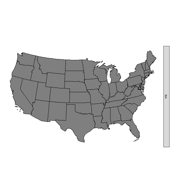
plot_usmap(data = dt, values = "value", exclude = c("AK", "HI"))+
   scale_fill_continuous(low = "white", high = "red", name = "Ele gen (EJ)", label = scales::comma)+ facet_grid("year")

这是最后的地图：

​

​

Answer 1

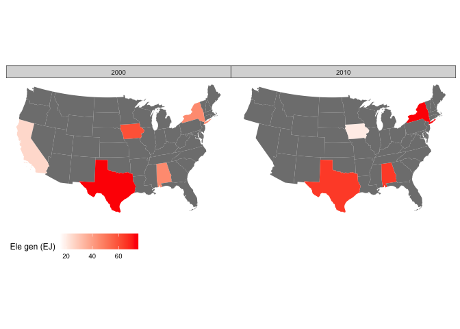
虽然plot_usmap使绘制快速地图变得很容易，但我认为，在您的示例中，使用ggplot2从头构建映射是可行的。

为此，您可以首先通过us_map获取原始地图数据，并将数据与地图数据合并。

但是，由于您的数据包含多年，但只有一些状态，所以我们必须“完成”数据集才能包含每一对年份和状态的观测结果。否则，按年计较是行不通的。为此，我首先按年份划分数据，将单个年份数据合并到地图数据，使用tidyr::fill填充年份列，最后按行绑定数据集：

dt <- data.frame(fips = c("CA", "AL", "NY","IA", "TX","CA", "AL", "NY","IA", "TX"),
                value = c(25, 45, 45, 60, 75,15, 65, 75, 20, 65),
                year=c(2000, 2000, 2000, 2000, 2000,2010, 2010, 2010, 2010, 2010))

library(usmap)
library(ggplot2)
library(dplyr)

# Map data
states <- us_map(exclude = c("AK", "HI"))

# Split, join, bind
states_data <- split(dt, dt$year) |> 
  lapply(function(x) left_join(states, x, by = c("abbr" = "fips"))) |> 
  lapply(function(x) tidyr::fill(x, year, .direction = "downup")) |> 
  bind_rows() |> 
  arrange(year, group, order)

ggplot(states_data, aes(x, y, fill = value, group = group)) +
  geom_polygon() +
  scale_fill_continuous(low = "white", high = "red", name = "Ele gen (EJ)", label = scales::comma) +
  facet_grid(~year) +
  coord_equal() +
  ggthemes::theme_map() +
  theme(legend.position = "bottom")

​

​

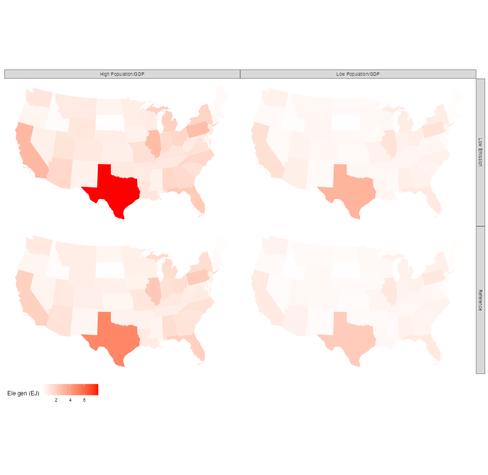
用所有状态的数据编辑真实数据的--数据准备要容易得多：

# Join and arrange
states_data <- left_join(states, dt, by = c("abbr" = "fips")) |> 
  arrange(emission, growth, group, order)

ggplot(states_data, aes(x, y, fill = value, group = group)) +
  geom_polygon() +
  scale_fill_continuous(low = "white", high = "red", name = "Ele gen (EJ)", label = scales::comma) +
  facet_grid(emission~growth) +
  coord_equal() +
  ggthemes::theme_map() +
  theme(legend.position = "bottom")

​

​